Main script
Note: Changes beyond this point are only needed if you are developing the notebook.
Initial settings.
First, we load the list of host land model variables that we may consider for the comparison.
source(file.path(util_path,"load.everything.r"),chdir=TRUE)We then make sure to set up the derived paths and files.
# Output path for time series.
comparison_path     = file.path(plot_main,"comparison"    )
taylor_biasvar_path = file.path(plot_main,"taylor_biasvar")

# Create output paths.
dummy = dir.create(comparison_path    ,recursive = TRUE,showWarnings = FALSE)
dummy = dir.create(taylor_biasvar_path,recursive = TRUE,showWarnings = FALSE)

# Define eddy covariance tower and leaf area index files.
site_path = file.path(site_main,case_site)
eddy_base = list.files(path=site_path,pattern="_eddy-summ\\.nc$")
mlai_base = list.files(path=site_path,pattern="_c6modis-summ\\.nc$")

#    Make sure we found the tower file, otherwise, stop. In case more than one file exists,
# we take the most recent one.
if (length(eddy_base) > 0){
   eddy_file = file.path(site_path,eddy_base)
   eddy_info = file.info(eddy_file)
   iuse      = which.max(as.POSIXct(eddy_info$mtime))
   eddy_base = eddy_base[iuse]
   eddy_file = eddy_file[iuse]
}else{
   cat(" Tower file data not found.  Check your settings.\n")
   cat(" site_main = \"",site_main,"\"\n",sep="")
   cat(" case_site = \"",case_site,"\"\n",sep="")
   cat(" site_path = \"",site_path,"\"\n",sep="")
   cat(" Path \"site_main\" exists = ",file.exists(site_main),"\n",sep="")
   cat(" Path \"site_path\" exists = ",file.exists(site_path),"\n",sep="")
   stop(" Path settings for site data are likely incorrect.")
}#end if


#    Make sure we found the MODIS LAI file, otherwise, skip LAI. In case more than one file exists,
# we take the most recent one.
if (length(mlai_base) > 0){
   mlai_file = file.path(site_path,mlai_base)
   mlai_info = file.info(mlai_file)
   iuse      = which.max(as.POSIXct(mlai_info$mtime))
   mlai_base = mlai_base[iuse]
   mlai_file = mlai_file[iuse]
}else{
   cat(" MODIS file data not found.  Check your settings.\n")
   cat(" site_main = \"",site_main,"\"\n",sep="")
   cat(" case_site = \"",case_site,"\"\n",sep="")
   cat(" site_path = \"",site_path,"\"\n",sep="")
   cat(" Path \"site_main\" exists = ",file.exists(site_main),"\n",sep="")
   cat(" Path \"site_path\" exists = ",file.exists(site_path),"\n",sep="")
   warning(" MODIS data are not available for this site.")
}#end if
Next, we find the correct simulation path. We search for files in the typical paths in which ELM-FATES or CLM-FATES simulations would be located. We also set the times for which we will retrieve simulation results. A few noteworthy variables.
- tstamp0. First simulation time. This is always the actual first output file of the simulation, because the first output always has additional variables that are useful for analyses.
- tstampa. First time used for output. If
case_tstampawas set asNA_character_at the beginning of the script, we will use the first available time. - tstampz. Last time used for output. If
thiscase_tstampzwas set asNA_character_` at the beginning of the script, we will use the last available time. - tstamp. The vector with all times that should be loaded.
- ntstamp. The total count of time steps to load.
cat0(" + Search FATES output.")

# List of HLM "mid-fixes" (like a prefix or suffix, but in the middle...)
hlm_midfix_lookup = c("elm.h0","clm2.h0")


# Expand variable case_info (or reset variables if they already exist.)
case_info = case_info %>%
            mutate( tstamp_1st = ""
                  , tstamp_lst = ""
                  , year0      = NA_integer_
                  , month0     = NA_integer_
                  , yeara      = NA_integer_
                  , montha     = NA_integer_
                  , yearz      = NA_integer_
                  , monthz     = NA_integer_
                  , hlm_midfix = ""
                  , simul_path = ""
                  , nc_zero    = "" )

# Extract scalars.
for (i in sequence(n_case_info)){
   # Extract scalars
   case_name    = case_info$name   [i]
   case_model   = case_info$model  [i]
   case_desc    = paste0(case_info$desc[i]," (",case_model,")")
   case_site    = case_info$site   [i]
   case_tstampa = case_info$tstampa[i]
   case_tstampz = case_info$tstampz[i]
   cat0("   - ",case_name,".")

   # Case path and possible simulation paths.  Do not change this unless you used non-standard case output for ELM/CLM.
   case_path = file.path(hesm_main,case_name)
   simul_path = c( file.path(case_path,"run"), file.path(case_path,"lnd","hist"))

   #---~---
   #    Vector with all possible ELM/CLM paths containing NetCDF history files.  Do not change
   # this unless you know what you are doing.
   #---~---
   nc_base    = paste0(case_name[1],".",hlm_midfix_lookup,"\\.....-..\\.nc")
   nc_file    = file.path( rep(x = simul_path, times = length(nc_base   ))
                         , rep(x = nc_base   , each  = length(simul_path))
                         )#end file.path
   nc_success = FALSE
   for (d in seq_along(nc_file)){
      nc_path = dirname(nc_file[d])
      nc_base = basename(nc_file[d])
      nc_list = list.files(path=nc_path,pattern=nc_base)
      if (length(nc_list) > 0){
         # When finding the files, update nc_success find the first and last time.
         nc_success = TRUE

         # Find file name and the length of each file
         nc_nfile = length(nc_list)
         nc_nchar = nchar(nc_list[1])

         # Find all times
         nc_year   = as.numeric(substring(nc_list,nc_nchar-9,nc_nchar-6))
         nc_month  = as.numeric(substring(nc_list,nc_nchar-4,nc_nchar-3))
         nc_tstamp = make_datetime(year=nc_year,month=nc_month)

         # Find the first and last time available.
         i1st                    = which.min(nc_tstamp)
         ilst                    = which.max(nc_tstamp)
         nc_t1st                 = nc_tstamp[i1st]
         nc_tlst                 = nc_tstamp[ilst]
         case_info$tstamp_1st[i] = sprintf("%2.2i/%2.2i/%4.4i",month(nc_t1st),day(nc_t1st),year(nc_t1st))
         case_info$tstamp_lst[i] = sprintf("%2.2i/%2.2i/%4.4i",month(nc_tlst),day(nc_tlst),year(nc_tlst))
         case_info$year0     [i] = year(nc_t1st)
         case_info$month0    [i] = month(nc_t1st)


         # Save the path and "midfix" that worked.
         case_info$simul_path[i] = nc_path
         case_info$nc_zero   [i] = file.path(nc_path,nc_list[1])
         sel_midfix              = mapply(FUN=grepl,pattern=as.list(hlm_midfix_lookup),MoreArgs=list(x=nc_base))
         case_info$hlm_midfix[i] = hlm_midfix_lookup[sel_midfix]

         if (is.na(case_tstampa)){
            case_info$yeara  [i] = year(nc_t1st)
            case_info$montha [i] = month(nc_t1st)
         }else{
            tstampa              = as.integer(unlist(strsplit(case_tstampa,split="/")))
            case_info$yeara  [i] = tstampa[3]
            case_info$montha [i] = tstampa[1]
         }#end if (is.character(tstampa))
         if (is.na(case_tstampz)){
            case_info$yearz  [i] = year(nc_tlst)
            case_info$monthz [i] = month(nc_tlst)
         }else{
            tstampz              = as.integer(unlist(strsplit(case_tstampz,split="/")))
            case_info$yearz  [i] = tstampz[3]
            case_info$monthz [i] = tstampz[1]
         }#end if (is.character(tstampz))


      }#end if (length(nc_list) > 0)
   }#end for (d in seq_along(nc_file))
}#end for for (i in sequence(n_case_info))
Find time settings common to all simulations. We always select the time intersection to make the best
# Create lubridate object for initial and final time. We select the time intersection
tstampa = max(make_datetime( year=case_info$yeara,month=case_info$montha,day=1L))
yeara   = year (tstampa)
montha  = month(tstampa)
tstampz = min(make_datetime( year=case_info$yearz,month=case_info$monthz,day=1L))
yearz   = year (tstampz)
monthz  = month(tstampz)

# Useful variables to build time stamps.
nmontha   = 12 - montha + 1          # Number of months in yeara
nmidyears = max(0,yearz - yeara - 1) # Number of years in between yeara and yearz
nmonthz   = monthz                   # Number of months in yearz

# Create month and year vector
if (yeara == yearz){
   # Simulation did not last more than one year
   tmonth = seq(from=montha,to=monthz,by=1)
   tyear  = rep(x=yeara,times=length(tmonth))
}else{
   # Simulation lasted longer than a year.
   tmonth = c( seq(from=montha,to=12,by=1)
             , rep(sequence(12),times=nmidyears)
             , seq(from=1     ,to=monthz,by=1)
             )#end c
   tyear  = c( rep(yeara,each=nmontha)
             , rep(yeara+sequence(nmidyears),each=12)
             , rep(yearz,each=nmonthz)
             )#end c
}#end if (yeara == yearz)

# Create time stamp and find how many times should be processed.
tstamp = make_datetime(year=tyear,month=tmonth,day=1L)
ntstamp = length(tstamp)
Data retrieval.
First we retrieve the site measurements and estimates of ecosystem productivity and respiration. Currently we only load simple time series, but in the future we may also consider canopy layer and soil measurements. Here we perform the following tasks:
- Load variables to be compared with the model.
- Apply unit conversion factors.
- Organise the data into a
tibbleobject.
For additional information on which variables to be loaded and which units to use in the output, check the hlm1dvar settings in RUtils/hlm_varlist.r.
if ("nc_eddy" %in% ls()){dummy = nc_close(nc_eddy); rm(nc_eddy)}

# Open NetCDF connection and retrieve variable names
cat0(" + Load site data from ",eddy_base,".")
nc_eddy  = nc_open(filename=eddy_file)
nc_nvars = nc_eddy$nvars
nc_ndims = nc_eddy$ndims
nc_dlist = rep(NA_character_,times=nc_ndims)
nc_vlist = rep(NA_character_,times=nc_nvars)
for (d in sequence(nc_ndims)) nc_dlist[d] = nc_eddy$dim[[d]]$name
for (v in sequence(nc_nvars)) nc_vlist[v] = nc_eddy$var[[v]]$name

# Select variables to load
nc_obs1d    = nc_vlist[tolower(nc_vlist) %in% hlm1dvar$vnam[hlm1dvar$assess]]


# Extract time information
eddy_time0  = as_datetime(gsub(pattern="^days since ",replacement="",x=nc_eddy$dim$time$units))
eddy_time   = eddy_time0 + days(nc_eddy$dim$time$vals)
n_eddy_time = nc_eddy$dim$time$len

# Initialise a tibble that will host all data
eddy1d = tibble( time = eddy_time, source = 0L)

# Find conversion factors for monthly variables.
cmon.day = days_in_month(eddy1d$time)
cmon.hr  = day.hr  * cmon.day
cmon.min = day.min * cmon.day
cmon.sec = day.sec * cmon.day

# Loop through variables, and load data sets.
o_loop = which(nc_obs1d %in% hlm1dvar$vnam)
for (o in seq_along(nc_obs1d)){
   # Retrieve settings for variable
   nc_nvnow        = nc_obs1d[o]
   h               = match(tolower(nc_nvnow),hlm1dvar$vnam)
   h_vnam          = hlm1dvar$vnam[h]
   h_desc          = hlm1dvar$desc[h]
   h_add0          = eval(parse(text=hlm1dvar$add0[h]))
   h_mult          = eval(parse(text=hlm1dvar$mult[h]))
   nc_dat          = ncvar_get(nc=nc_eddy,varid=nc_nvnow)
   cat0("   - Retrieve ",h_desc,".")
   eddy1d[[h_vnam]] = h_add0 + h_mult * nc_dat
}#end for (o in seq_along(nc_obs1d))

# Load site coordinates. We will check whether observations and model are reasonably close.
site_coord = tibble( clon = c(ncvar_get(nc=nc_eddy,varid="LONGXY"))
                   , clat = c(ncvar_get(nc=nc_eddy,varid="LATIXY"))
                   , wlon = c(ncvar_get(nc=nc_eddy,varid="EDGEW" ))
                   , elon = c(ncvar_get(nc=nc_eddy,varid="EDGEE" ))
                   , slat = c(ncvar_get(nc=nc_eddy,varid="EDGES" ))
                   , nlat = c(ncvar_get(nc=nc_eddy,varid="EDGEN" ))
                   )#end tibble


# Close file and remove connection.
dummy = nc_close(nc_eddy)
rm(nc_eddy)
If available, we retrieve MODIS-derived data. Currently only LAI is loaded, but other variables may be included in the future as well. For additional information on which variables to be loaded and which units to use in the output, check the fatesvar settings in RUtils/fates_varlist.r.
if (file.exists(mlai_file)){

   if ("nc_mlai" %in% ls()){dummy = nc_close(nc_mlai); rm(nc_mlai)}

   # Open NetCDF connection and retrieve variable names
   cat0(" + Load site data from ",mlai_base,".")
   nc_mlai  = nc_open(filename=mlai_file)
   nc_nvars = nc_mlai$nvars
   nc_ndims = nc_mlai$ndims
   nc_dlist = rep(NA_character_,times=nc_ndims)
   nc_vlist = rep(NA_character_,times=nc_nvars)
   for (d in sequence(nc_ndims)) nc_dlist[d] = nc_mlai$dim[[d]]$name
   for (v in sequence(nc_nvars)) nc_vlist[v] = nc_mlai$var[[v]]$name

   # Select variables to load
   nc_obs1d    = nc_vlist[tolower(nc_vlist) %in% hlm1dvar$vnam[hlm1dvar$assess]]


   # Extract time information
   mlai_time0  = as_datetime(gsub(pattern="^days since ",replacement="",x=nc_mlai$dim$time$units))
   mlai_time   = mlai_time0 + days(nc_mlai$dim$time$vals)
   n_mlai_time = nc_mlai$dim$time$len

   # Initialise a tibble that will host all data
   mlai1d = tibble( time = mlai_time, source = 0L)

   # Find conversion factors for monthly variables.
   cmon.day = days_in_month(mlai1d$time)
   cmon.hr  = day.hr  * cmon.day
   cmon.min = day.min * cmon.day
   cmon.sec = day.sec * cmon.day

   # Loop through variables, and load data sets.
   o_loop = which(nc_obs1d %in% hlm1dvar$vnam)
   for (o in seq_along(nc_obs1d)){
      # Retrieve settings for variable
      nc_nvnow        = nc_obs1d[o]
      h               = match(tolower(nc_nvnow),hlm1dvar$vnam)
      h_vnam          = hlm1dvar$vnam[h]
      h_desc          = hlm1dvar$desc[h]
      h_add0          = eval(parse(text=hlm1dvar$add0[h]))
      h_mult          = eval(parse(text=hlm1dvar$mult[h]))
      nc_dat          = ncvar_get(nc=nc_mlai,varid=nc_nvnow)
      cat0("   - Retrieve ",h_desc,".")
      mlai1d[[h_vnam]] = h_add0 + h_mult * nc_dat
   }#end for (o in seq_along(nc_obs1d))


   # Close file and remove connection.
   dummy = nc_close(nc_mlai)
   rm(nc_mlai)

   # Merge the two objects
   site1d      = full_join(x=eddy1d,y=mlai1d,by=c("time","source")) %>%
                 arrange(time,source)
   n_site_time = nrow(site1d)
}else{
   # MODIS data not found. Turn eddy1d into site1d.
   site1d = eddy1d
   n_site_time = n_eddy_time
}#end if (file.exists(mlai_file))
The time span for site simulations and tower may not match. In this case, we identify the overlapping time interval, and trim both the site and model assessment to this period in which both are available. We always keep track of the actual first time of the model, though, because the first history file contains additional data that may be useful when we adapt the code to compare soil state variables.
# Find the minimum interval that has overlaps with both site and model.
tstampa = max(c(min(tstamp),min(site1d$time)))
tstampz = min(c(max(tstamp),max(site1d$time)))

# Restrict time to the overlapping period
tstamp  = tstamp[(tstamp >= tstampa) & (tstamp <= tstampz)]
ntstamp = length(tstamp)

#   Trim site observations to the overlapping period. Also, standardise the data so we
# use only one of NA or NaN.
site1d = site1d %>%
         filter( (time >= tstampa) & (time <= tstampz)) %>%
         mutate_at(vars(-time),function(x) ifelse(is.nan(x),NA,x))
Here we perform the following tasks, using the actual first history file from the ELM/CLM simulation:
- Determine which path and file name structure .
- Initialise a
tibbleobject for all the candidate variables (Checkhlm1dvarsettings in RUtils/hlm_varlist.r for the list of variables). - Retrieve soil information (which will be useful when comparing the model against soil measurements).
- Retrieve size and PFT indices for the
_SCPFvariables (which will be useful in the future for comparing the model against census measurements).
if ("nc_info" %in% ls()){dummy = nc_close(nc_info); rm(nc_info)}


# Select the first case to retrieve general information on files
i            = 1
case_name    = case_info$name   [i]
case_model   = case_info$model  [i]
case_desc    = paste0(case_info$desc[i]," (",case_model,")")
case_site    = case_info$site   [i]
case_tstampa = case_info$tstampa[i]
case_tstampz = case_info$tstampz[i]
nc_zero      = case_info$nc_zero[i]


# We always read the first actual simulation time because it has more information.
# Open NetCDF connection and retrieve variable names
nc_info  = nc_open(filename=nc_zero)
nc_nvars = nc_info$nvars
nc_ndims = nc_info$ndims
nc_dlist = rep(NA_character_,times=nc_ndims)
nc_vlist = rep(NA_character_,times=nc_nvars)
for (d in sequence(nc_ndims)) nc_dlist[d] = nc_info$dim[[d]]$name
for (v in sequence(nc_nvars)) nc_vlist[v] = nc_info$var[[v]]$name

#---~---
# Gather variable information, then initialise tibble
#---~---

cat0("   - Identify all HLM variables.")
# Retrieve all "1D" variables that are available at the host model.
# A few variables may not exist in truly 1D, so we check if they may be reconstructed.
nc_pref   = tolower(x=nc_vlist)
nc_scpf   = ( nc_pref %in% paste0(hlm1dvar$vnam,"_canopy_scpf"    )
            | nc_pref %in% paste0(hlm1dvar$vnam,"_understory_scpf") )
nc_scls   = ( nc_pref %in% paste0(hlm1dvar$vnam,"_canopy_scls"    )
            | nc_pref %in% paste0(hlm1dvar$vnam,"_understory_scls") )
nc_keep   = nc_pref %in% hlm1dvar$vnam | ( ( !  nc_pref %in% hlm1dvar$vnam ) & ( nc_scpf | nc_scls ) )
no_hlm1d  = nc_vlist[! nc_keep]
nc_hlm1d  = nc_vlist[  nc_keep]

# Remove suffix, we will add them back later when needed.
nc_hlm1d  = gsub(pattern="_CANOPY_SCPF$"    ,replacement="",x=nc_hlm1d)
nc_hlm1d  = gsub(pattern="_CANOPY_SCLS$"    ,replacement="",x=nc_hlm1d)
nc_hlm1d  = gsub(pattern="_UNDERSTORY_SCPF$",replacement="",x=nc_hlm1d)
nc_hlm1d  = gsub(pattern="_UNDERSTORY_SCLS$",replacement="",x=nc_hlm1d)
nc_hlm1d  = sort(unique(nc_hlm1d))

# Check whether to append "evapotranspiration"
cat("   - Check whether or not we can find evapotranspiration... ")
if (  ( all(c("QSOIL","QVEGT","QVEGE") %in% nc_hlm1d) ) && (! "QEVTR" %in% nc_hlm1d) ){
   nc_hlm1d = unique(c(nc_hlm1d,"QEVTR"))
   etr_last = TRUE
   cat0("  Yes!")
}else{
   etr_last = FALSE
   cat0("  No!")
}#end if (  ( all(c("QSOIL","QVEGT","QVEGE") %in% nc_hlm1d) ) && (! "QEVTR" %in% nc_hlm1d) )

# Check whether to append ecosystem respiration
cat("   - Check whether or not we can find ecosystem respiration... ")
if (  ( all(c("AR","HR") %in% nc_hlm1d) ) && (! "ER" %in% nc_hlm1d) ){
   nc_hlm1d = unique(c(nc_hlm1d,"ER"))
   er_last  = TRUE
   cat0("  Yes!")
}else{
   er_last  = FALSE
   cat0("  No!")
}#end if (  ( all(c("AR","HR") %in% nc_hlm1d) ) && (! "ER" %in% nc_hlm1d) )

# Find number of host land model variables
nhlm1d    = length(nc_hlm1d)


# Initialise 1D variables available at the HLM
cat0("   - Initialise tibble for the host land model.")
hlm1d = tibble( time   = rep(tstamp,times=n_case_info)
              , source = rep(sequence(n_case_info),each=ntstamp)
              )#end tibble
for (h in seq_along(nc_hlm1d)){
   h_vnam          = tolower(nc_hlm1d[h])
   hlm1d[[h_vnam]] = rep(NA,times=ntstamp*n_case_info)
}#end for (h in seq_along(nc_hlm1d))


# Load simulation coordinates. We check whether observations and model are reasonably close.
hlm1d_coord = tibble( clon = c(ncvar_get(nc=nc_info,varid="lon"))
                    , clat = c(ncvar_get(nc=nc_info,varid="lat"))
                    )#end tibble
lon_fine = hlm1d_coord$clon >= site_coord$wlon && hlm1d_coord$clon <= site_coord$elon
lat_fine = hlm1d_coord$clat >= site_coord$slat && hlm1d_coord$clat <= site_coord$nlat
if (! all(c(lon_fine,lat_fine))){
   cat0("------------------------------------------------------------------")
   cat0(" Simulation and site information are not from the same location.  ")
   cat0(" ")
   cat0(" Site")
   cat0(" Longitude:               ",site_coord$clon)
   cat0(" Latitude:                ",site_coord$clat)
   cat0(" Zonal grid extent:      (",site_coord$wlon,";",site_coord$elon,")")
   cat0(" Meridional grid extent: (",site_coord$slat,";",site_coord$nlat,")")
   cat0(" ")
   cat0(" Model")
   cat0(" Longitude:               ",hlm1d_coord$clon)
   cat0(" Latitude:                ",hlm1d_coord$clat)
   cat0("------------------------------------------------------------------")
   stop(" Model coordinates must be within the site grid extent.")
}#end if (! all(c(lon_fine,lat_fine)))

# Close connection
dummy   = nc_close(nc_info)
We also read the soil information and the indices for PFT and size classes. Because these quantities may vary across simulations depending on the scientific question, we load all of them and save in lists. Currently this is not used but could be important in the future, if soil variables or census variables are compared.
# For soil layers and size-pft indices, we save a list for each simulation, as the PFT definitions and soil depth may vary across simulations.
slayer     = list()
index_scpf = list()
for (i in sequence(n_case_info)){
   # Select the first case to retrieve general information on files
   case_name    = case_info$name   [i]
   case_model   = case_info$model  [i]
   case_desc    = paste0(case_info$desc[i]," (",case_model,")")
   case_site    = case_info$site   [i]
   case_tstampa = case_info$tstampa[i]
   case_tstampz = case_info$tstampz[i]
   nc_zero      = case_info$nc_zero[i]
   cat0(" + Load additional information: ",case_name,".")

   # We always read the first actual simulation time because it has more information.
   # Open NetCDF connection and retrieve variable names
   nc_info  = nc_open(filename=nc_zero)
   nc_nvars = nc_info$nvars
   nc_ndims = nc_info$ndims
   nc_dlist = rep(NA_character_,times=nc_ndims)
   nc_vlist = rep(NA_character_,times=nc_nvars)
   for (d in sequence(nc_ndims)) nc_dlist[d] = nc_info$dim[[d]]$name
   for (v in sequence(nc_nvars)) nc_vlist[v] = nc_info$var[[v]]$name


   # Load soil layers.  This is currently not used, but could be used for soil comparisons.
   cat0("   - Load soil information")
   slayer[[case_name]] = tibble( zsoi   = c(unlist(ncvar_get(nc=nc_info,varid='ZSOI'  )))
                               , dzsoi  = c(unlist(ncvar_get(nc=nc_info,varid='DZSOI' )))
                               , bsw    = c(unlist(ncvar_get(nc=nc_info,varid='BSW'   )))
                               , hksat  = c(unlist(ncvar_get(nc=nc_info,varid='HKSAT' )))
                               , sucsat = c(unlist(ncvar_get(nc=nc_info,varid='SUCSAT')))
                               , watsat = c(unlist(ncvar_get(nc=nc_info,varid='WATSAT')))
                               )#end data.table

   #---~---
   #    Load size and PFT indices. This is currently not used, but could be used for
   # census comparisons.
   #---~---
   cat0("   - Load indices for size- and pft-dependent variables.")
   index_scpf[[case_name]] = tibble( scls   = ncvar_get(nc=nc_info,varid='fates_scmap_levscpf'  )
                                   , pft    = ncvar_get(nc=nc_info,varid='fates_pftmap_levscpf' )
                                   )#end tibble

   # Close connection
   dummy   = nc_close(nc_info)

}#end for (i in sequence(n_case_info))
We now go through every monthly output file to retrieve the averages by month and year. Specifically, we do the following: 1. Load all the 1-D variables available in the history file and defined in the hlm1dvar object (see RUtils/hlm_varlist.r). 2. Apply unit conversion factors. 3. Find derived variables that are not directly available in the history files (currently evapotranspiration and ecosystem respiration). 4. Organise the data into a tibble object.
if ("nc_hlm" %in% ls()){dummy = nc_close(nc_hlm); rm(nc_hlm)}

for (i in sequence(n_case_info)){
   # Select the first case to retrieve general information on files
   case_name    = case_info$name      [i]
   case_model   = case_info$model     [i]
   case_desc    = paste0(case_info$desc[i]," (",case_model,")")
   case_site    = case_info$site      [i]
   case_tstampa = case_info$tstampa   [i]
   case_tstampz = case_info$tstampz   [i]
   nc_zero      = case_info$nc_zero   [i]
   simul_path   = case_info$simul_path[i]
   hlm_midfix   = case_info$hlm_midfix[i]
   cat0(" + Load model output: ",case_name,".")


   for (w in sequence(ntstamp)){
      # Extract times and build file name
      w_month  = month(tstamp[w])
      w_year   = year (tstamp[w])
      w_ymlab  = sprintf("%4.4i-%2.2i",w_year,w_month)
      nc_base  = paste0(case_name,".",hlm_midfix,"." ,w_ymlab,".nc")
      nc_file  = file.path(simul_path,nc_base)
      cat0("   - Retrieve file ",nc_base,".")


      # Find conversion factors for monthly variables.
      cmon.day = days_in_month(tstamp[w])
      cmon.hr  = day.hr  * cmon.day
      cmon.min = day.min * cmon.day
      cmon.sec = day.sec * cmon.day


      # Open NetCDF connection and retrieve variable names
      nc_hlm   = nc_open(filename=nc_file)

      # Read 1D variables
      for (v in sequence(nhlm1d-etr_last-er_last)){
         # Retrieve variable
         nc_nvnow            = nc_hlm1d[v]
         nc_can_scpf         = paste0(nc_nvnow,"_CANOPY_SCPF")
         nc_und_scpf         = paste0(nc_nvnow,"_UNDERSTORY_SCPF")
         nc_can_scls         = paste0(nc_nvnow,"_CANOPY_SCLS")
         nc_und_scls         = paste0(nc_nvnow,"_UNDERSTORY_SCLS")
         nc_pref             = tolower(x=nc_nvnow)

         # Map variable to variable table, get the addition and multiplication factors.
         h                   = match(nc_pref,hlm1dvar$vnam)
         h_vnam              = hlm1dvar$vnam[h]
         h_add0              = eval(parse(text=hlm1dvar$add0[h]))
         h_mult              = eval(parse(text=hlm1dvar$mult[h]))

         # Find line for current time and simulation.
         iw                  = which( ( hlm1d$time %eq% tstamp[w]) & (hlm1d$source %eq% i) )

         # Decide how to populate the variable
         if (nc_nvnow %in% nc_vlist){
            # Read variable as is.
            nc_dat               = ncvar_get(nc=nc_hlm,varid=nc_nvnow)
            hlm1d[[h_vnam]][iw]  = h_add0 + h_mult * nc_dat
         }else if(all(c(nc_can_scpf,nc_und_scpf) %in% nc_vlist)){
            # Build variable from the size- and PFT- arrays.
            nc_can               = ncvar_get(nc=nc_hlm,varid=nc_can_scpf)
            nc_und               = ncvar_get(nc=nc_hlm,varid=nc_und_scpf)
            hlm1d[[h_vnam]][iw]  = h_add0 + h_mult * sum(nc_can+nc_und)
         }else if(all(c(nc_can_scls,nc_und_scls) %in% nc_vlist)){
            # Build variable from the size- and PFT- arrays.
            nc_can               = ncvar_get(nc=nc_hlm,varid=nc_can_scls)
            nc_und               = ncvar_get(nc=nc_hlm,varid=nc_und_scls)
            hlm1d[[h_vnam]][iw]  = h_add0 + h_mult * sum(nc_can+nc_und)
         }else{
            cat0("--------------------------------------------------")
            cat0(" The following variable is not available: ",nc_nvnow,".")
            cat0(" The attempts to add canopy and under storey also failed..")
            stop(" Missing variable.")
         }#end if (is.na(h))
      }#for (h in sequence(nhlm1d-etr_last-et_last))

      # Find total ET.
      if (etr_last){
         hlm1d$qevtr[iw] = hlm1d$qvege[iw] + hlm1d$qvegt[iw] + hlm1d$qsoil[iw]
      }#end if (etr_last)

      # Find total ET.
      if (er_last){
         hlm1d$er[iw] = hlm1d$ar[iw] + hlm1d$hr[iw]
      }#end if (er_last)

      # Close connection
      dummy   = nc_close(nc_hlm)
   }#end for (w in sequence(nstamp))

}#end for (i in sequence(n_case_info))
We now compare the variables from the site measurements and the model, and keep only the variables present in both data sets.
cat0(" + Find the variables common to both site and model.")
# Find common variables
var_both = intersect(names(site1d),names(hlm1d))
var_both = var_both[! var_both %in% c("time","source")]

# Restrict variables for both site and model
site1d = site1d %>% select( all_of(c("time","source",var_both)))
hlm1d  = hlm1d  %>% select( all_of(c("time","source",var_both)))
Combine site and model into a single object (emean), then we calculate mean seasonality and the range (mmean).
# Merge data sets, we set 1 for site measurements, and 2 for the host model.
cat0(" + Merge data sets into a single tibble.")
emean  = rbind( site1d, hlm1d) %>%
         select(all_of(c("time","source",var_both))) %>%
         filter( ( time %in% unique(site1d$time) )
               & ( time %in% unique(hlm1d$time ) ) )

# Find the mean seasonal cycle.
mmean = emean                                                             %>%
        mutate( year = year(time), month = month(time))                   %>%
        group_by(month,source)                                            %>%
        select(! c(time,year))                                            %>%
        summarise_all(mean, na.rm=TRUE)                                   %>%
        ungroup()                                                         %>%
        rename_at(vars(var_both), function(x) paste0(x,"_mean"))

# Find the lower range of the seasonal cycle
mqlwr = emean                                                             %>%
        mutate( year = year(time), month = month(time))                   %>%
        group_by(month,source)                                            %>%
        select(! c(time,year))                                            %>%
        summarise_all(quantile,probs=qlwr_ribbon,names=FALSE, na.rm=TRUE) %>%
        ungroup()                                                         %>%
        rename_at(vars(var_both), function(x) paste0(x,"_qlwr"))

# Find the upper range of the seasonal cycle
mqupr = emean                                                             %>%
        mutate( year = year(time), month = month(time))                   %>%
        group_by(month,source)                                            %>%
        select(! c(time,year))                                            %>%
        summarise_all(quantile,probs=qupr_ribbon,names=FALSE, na.rm=TRUE) %>%
        ungroup()                                                         %>%
        rename_at(vars(var_both), function(x) paste0(x,"_qupr"))

# Find the annual averages.
mmean = as_tibble( merge( x  = merge(x=mmean,y=mqlwr,by=c("month","source"))
                        , y  = mqupr
                        , by = c("month","source")
                        )#end merge
                 )#end as_tibble

# Sort data by month and source
mmean = mmean %>% arrange(source,month)
Simple model evaluation plots
First, we plot the time series of monthly averages for both site measurements (or estimates) and model predictions.
cat0(" + Plot time series comparisons between site measurements/estimates and model predictions.")


# Set legends
leg_colours = c(site_colour,case_info$colour)
leg_labels  = c("Site",paste0(case_info$model,": ",case_info$desc))

gg_emean = list()
for (v in seq_along(var_both)){
   # Load variable
   h        = match(var_both[v],hlm1dvar$vnam)
   h_vnam   = hlm1dvar$vnam [h]
   h_desc   = hlm1dvar$desc [h]
   h_short  = hlm1dvar$short[h]
   h_unit   = hlm1dvar$unit [h]
   h_legend = v == 1


   # Temporary data table. We convert the classes back to factor.
   h_emean        = emean
   h_emean$source = factor(h_emean$source,levels=unique(h_emean$source))

   # Initialise plot (we use line)
   gg_now = ggplot(data=h_emean,aes_string(x="time",y=h_vnam,group="source",colour="source"))
   gg_now = gg_now + scale_colour_manual(name="",labels=leg_labels,values=leg_colours)

   # We only add legend for a single plot.  Patchwork will fix this in the end.
   gg_now = gg_now + geom_line(lwd=0.8,show.legend = h_legend)

   # Add local annotation
   gg_now = gg_now + labs(title=element_blank())
   gg_now = gg_now + scale_x_datetime(date_labels=gg_tfmt)
   gg_now = gg_now + xlab(element_blank())
   gg_now = gg_now + ylab(desc.unit(desc=h_short,unit=untab[[h_unit]],dxpr=TRUE))
   gg_now = gg_now + theme_grey( base_size      = gg_ptsz
                               , base_family    = "Helvetica"
                               , base_line_size = 0.5
                               , base_rect_size = 0.5
                               )#end theme_grey

   # Additional legend settings
   # if (h_legend) gg_now = gg_now + theme( legend.position = "bottom")

   # Axis settings
   gg_now = gg_now + theme( axis.text.x       = element_text( size   = gg_ptsz
                                                            , margin = unit(rep(0.35,times=4),"char")
                                                            )#end element_text
                          , axis.text.y       = element_text( size   = gg_ptsz
                                                            , margin = unit(rep(0.35,times=4),"char")
                                                            )#end element_text
                          , axis.ticks.length = unit(-0.2,"char")
                          , axis.title.y      = element_text( size = gg_ptsz * 0.9)
                          , legend.text       = element_text( size = gg_ptsz * 0.7)
                          )#end theme

  # Write plot settings to the list.
  gg_emean[[h_vnam]] = gg_now
}#end for (v in seq_along(var_both)){

# Wrap plots then global settings and x axis.
gg_patch = wrap_plots(gg_emean)
gg_patch = gg_patch + guide_area() + plot_layout(guides="collect")
gg_patch = gg_patch + plot_annotation(tag_levels = "a", title = case_pref)

# Save plots.
for (d in sequence(ndevice)){
   h_output = paste0("comparison_tseries-",case_pref,".",gg_device[d])
   dummy    = ggsave( filename = h_output
                    , plot     = gg_patch
                    , device   = gg_device[d]
                    , path     = comparison_path
                    , width    = gg_width
                    , height   = gg_height
                    , units    = gg_units
                    , dpi      = gg_depth
                    )#end ggsave

}#end for (d in sequence(ndevice))

# If sought, plot images on screen
if (gg_screen) plot(gg_patch)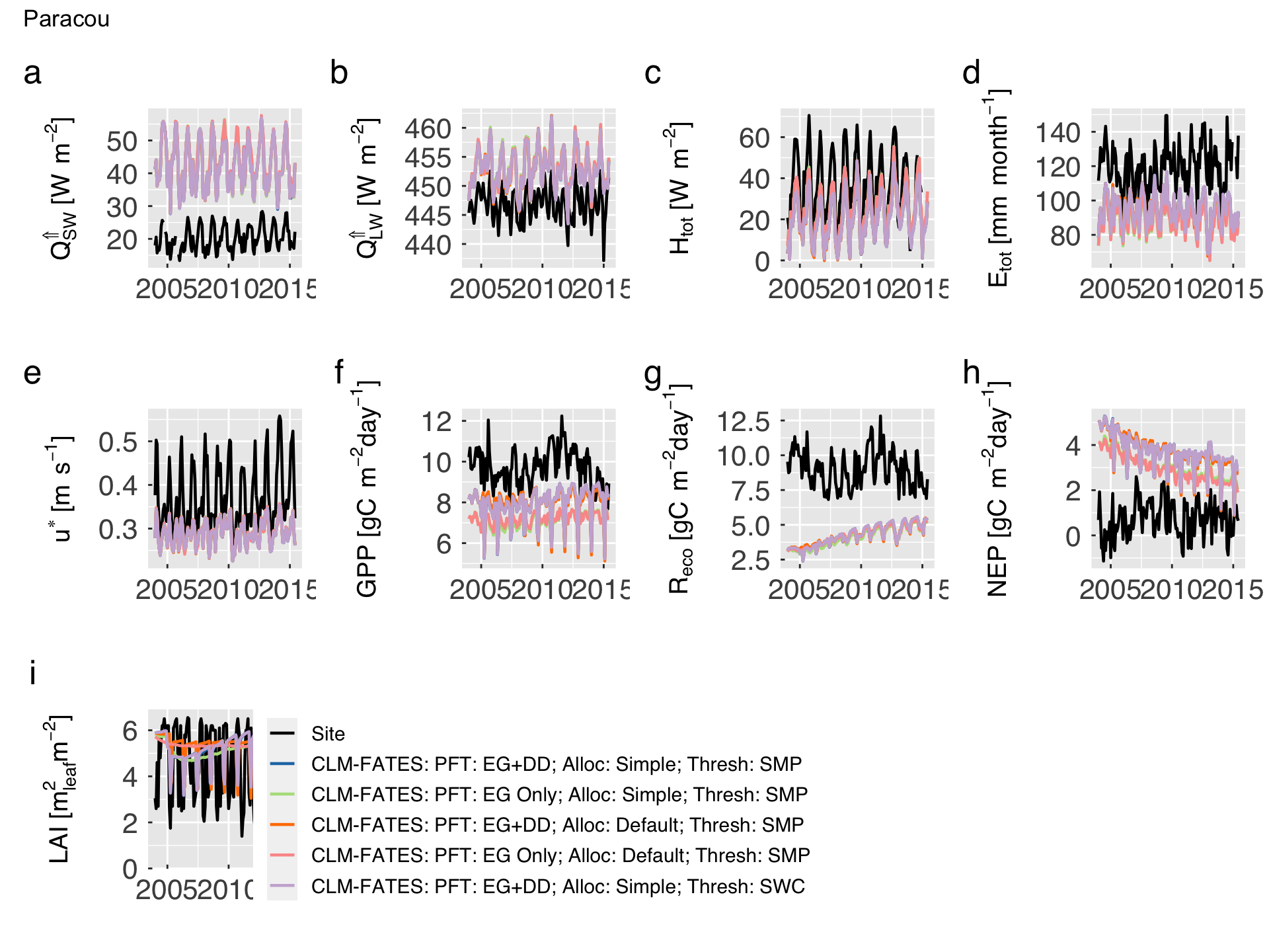
Then we plot the mean seasonal cycle for both site measurements/estimates and model predictions. We also include a 68% inter-annual variability band.
cat0(" + Plot the mean seasonal cycle of site measurements/estimates and model predictions.")

# Set legends
leg_colours = c(site_colour,case_info$colour)
leg_labels  = c("Site",paste0(case_info$model,": ",case_info$desc))

gg_emean = list()
for (v in seq_along(var_both)){
   # Load variable
   h        = match(var_both[v],hlm1dvar$vnam)
   h_vnam   = hlm1dvar$vnam [h]
   h_vmean  = paste0(h_vnam,"_mean")
   h_vqlwr  = paste0(h_vnam,"_qlwr")
   h_vqupr  = paste0(h_vnam,"_qupr")
   h_desc   = hlm1dvar$desc [h]
   h_short  = hlm1dvar$short[h]
   h_unit   = hlm1dvar$unit [h]
   h_legend = v == 1


   # Temporary data table. We convert the classes back to factor.
   h_mmean        = mmean
   h_mmean$source = factor(h_mmean$source,levels=unique(h_mmean$source))

   # Initialise plot (we use line)
   gg_now = ggplot( data    = h_mmean
                  , mapping = aes_string( x      = "month"
                                        , group  = "source"
                                        , colour = "source"
                                        , fill   = "source"
                                        )
                  )#end ggplot
   gg_now = gg_now + scale_colour_manual(name="",aesthetics="colour",labels=leg_labels,values=leg_colours)
   gg_now = gg_now + scale_colour_manual(name="",aesthetics="fill"  ,labels=leg_labels,values=leg_colours)

   # We only add legend for a single plot.  Patchwork will fix this in the end.
   gg_now = gg_now + geom_ribbon( aes_string(ymin=h_vqlwr,ymax=h_vqupr)
                                , alpha       = alpha_ribbon
                                , show.legend = h_legend
                                , colour      = "transparent"
                                )#end geom_ribbon
   gg_now = gg_now + geom_line( aes_string(y=h_vmean)
                              , lwd = 0.8
                              , show.legend = h_legend
                              )#end geom_line


   # Add local annotation
   gg_now = gg_now + labs(title=element_blank())
   gg_now = gg_now + scale_x_continuous( breaks = sequence(12)
                                       , labels = substring(month.abb,1,1)
                                       )#end scale_x_continuous
   gg_now = gg_now + xlab(element_blank())
   gg_now = gg_now + ylab(desc.unit(desc=h_short,unit=untab[[h_unit]],dxpr=TRUE))
   gg_now = gg_now + theme_grey( base_size      = gg_ptsz
                               , base_family    = "Helvetica"
                               , base_line_size = 0.5
                               , base_rect_size = 0.5
                               )#end theme_grey

   # Additional legend settings
   # if (h_legend) gg_now = gg_now + theme( legend.position = "bottom")

   # Axis settings
   gg_now = gg_now + theme( axis.text.x       = element_text( size   = gg_ptsz
                                                            , margin = unit(rep(0.35,times=4),"char")
                                                            )#end element_text
                          , axis.text.y       = element_text( size   = gg_ptsz
                                                            , margin = unit(rep(0.35,times=4),"char")
                                                            )#end element_text
                          , axis.ticks.length = unit(-0.2,"char")
                          , axis.title.y      = element_text( size = gg_ptsz * 0.9)
                          , legend.text       = element_text( size = gg_ptsz * 0.7)
                          )#end theme

  # Write plot settings to the list.
  gg_emean[[h_vnam]] = gg_now
}#end for (v in seq_along(var_both)){

# Wrap plots then global settings and x axis.
gg_patch = wrap_plots(gg_emean)
gg_patch = gg_patch + guide_area() + plot_layout(guides="collect")
gg_patch = gg_patch + plot_annotation(tag_levels = "a", title = case_pref)

# Save plots.
for (d in sequence(ndevice)){
   h_output = paste0("comparison_meanseason-",case_pref,".",gg_device[d])
   dummy    = ggsave( filename = h_output
                    , plot     = gg_patch
                    , device   = gg_device[d]
                    , path     = comparison_path
                    , width    = gg_width
                    , height   = gg_height
                    , units    = gg_units
                    , dpi      = gg_depth
                    )#end ggsave

}#end for (d in sequence(ndevice))

# If sought, plot images on screen
if (gg_screen) gg_patch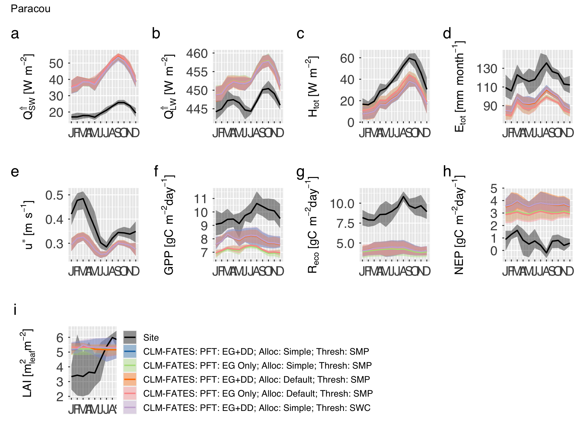
Taylor and bias-variance diagrams
We now generate a few summary diagrams that allow us to compare the model behaviour for all the variables in the same plot. First, we must first combine all the variables in rows, and leave observations and models in separate columns.
# Re-arrange site data for the Taylor diagram
td0_site = emean %>%
           filter(source == 0) %>%
           melt(id.vars=c("time","source"),measure.vars=var_both,variable.factor=FALSE,value.name="site") %>%
           as_tibble()

# Create tiblle with as many observations as models
td_site = NULL
for (i in sequence(n_case_info)){
   td_site = rbind(td_site,  td0_site %>% mutate(source = i))
}#end for (i in sequence(n_case_info))


# Re-arrange model data for the Taylor diagram
td_model  = emean %>%
            filter(source != 0) %>%
            melt(id.vars=c("time","source"),measure.vars=var_both,variable.factor=FALSE,value.name="model") %>%
            as_tibble()


# Find factor names
v_short = hlm1dvar$short[match(var_both,hlm1dvar$vnam)]

# Combine both data sets.
td_data = as_tibble(merge(x=td_site,y=td_model,by=c("time","source","variable"))) %>%
          arrange(variable,time) %>%
          mutate( variable = factor(variable) )

# Create tibble with model configurations
td_config = td_data %>%
            mutate( source = factor(case_info$name[source],levels=case_info$name) ) %>%
            pivot_wider(names_from="source",values_from="model")


#    Split data into seasons, using a simple function. We use the month acronyms so it works
# for both hemispheres.
which_season  = function(x){
   sref = rep(c("DJF","MAM","JJA","SON"),each=3)
   sref=c(sref[-1],sref[1])
   ans = sref[month(x)]
   return(ans)
}#end function (which_season)
td_data = td_data %>% mutate(season = which_season(time))

# Create tibble with seasons as separate models.
td_season = td_data %>% pivot_wider(names_from="season",values_from="model")
Generate the Taylor diagrams accounting for all variables and separating by season. Multiple model runs can be also provided for model improvement assessment. This is done by function RUtils/gg_taylor.r). This function is based on plotrix::taylor.diagram, but incorporating more tidyverse elements.
Inputs
x. Data set (data.frame,data.table, ortibble), it can be coerced to tibble. It is often necessary to rearrange the data, check functionsdata.table::meltanddplyr::pivot_longerwhich may help.obser. Column inxthat represents the observations. Default is"obs". This column may contain multiple variables, sites, seasons, or other category, as long as they can be identified by another column inx.model. Column(s) inxthat represents the model results. Default is a single column named"mod". Each row should correspond to the equivalent value inobser.group. Column inxthat describes how to classify the data. Each group will have a specific colour in the diagram. If none is provided, a single point will be pooled.panel. Column inxthat describes how to split the data. Each panel will be plot in a separate sub-figure in the diagram. If none is provided, a single panel will be plot.model_optsandgroup_opts. List of options for handling model/group annotation in the legend (used only if more than one model/group exists):title. Title for legend caption.label. Labels for models or groups. In the case of model_opts, this must have the same length as variable model. In the case of group_opts, this must match the number of unique groups. Iflabelis not provided, the code will use the same category names as variable model. If variablegroupis a character, we strongly recomend to use a named vector in which the names match the values in the group column (e.g.group_label = c(class_a = "A", class_b = "B").
colour_opts. List of options for colours. The following elements can be provided:by. In case multiple models and groups are provided, usebyto indicate which dimension should be distinguished by colour. Options are"model"or"group". The other one will be distinguished by shape. In case only one of them have multiple categories, we ignorebyand use both shape and colours to distinguish the categories.level. Colours for the categories distinguished by shapes. IfNULL, the colours will be automatically assigned. Otherwise, this can be a palette from packageRColorBrewer, a palette in packageviridis, a function that takes the number of sought colours as the first argument, or a vector with as many colours as categories.reverse. In case colour is a palette or function, reverse it?
shape_opts. List of options for shapes. The following elements can be provided:level. List of shapes for the categories distinguished by shapes. It can be a vector of numbers (same as those defined by lty) or characters (similar toggplot), with as many elements as categories. IfNULL, the shapes will be automatically assigned. Important: avoid using many more than 6 shapes because it makes the plot difficult to read.solid. In case shape isNULL, use solid shapes (TRUE or FALSE).size. Size for symbols.
panel_opts. List with options for panels. The following elements can be provided:label. Labels, to appear in the sub-plot titles (used only if more than one panel exists). This must match the number of unique groups. If none is provided, the code will use the unique values in variable panel. If variable group is a character, we strongly recomend to use a named vector in which the names match the values in the panel column (e.g.label = c(class_a = "A", class_b = "B")).levels. Type of level to use for panel annotation tags. This follows the same idea ofpatchwork::plot_annotation. Options are"a"for lowercase letters,"A"for uppercase letters,"1"for numbers,"i"for lowercase Roman numerals,"I"for uppercase Roman numerals. Empty character will skip levels.prefix. String to appear before the tag.suffix. String to appear after the tag and before the panel labels.sep. Separator between tag, prefix, and suffix. There will be always a space between tag and labels if panel_levels is not empty.
axis_opts. List of options for the main axes.colour. Colour for main axes.linetype. Line type for main axes.size. Line width for main axes.
sigma_opts,corr_opts,gamma_opts. List of options for the standard deviation of the model (sigma), correlation between model and observations (corr), and standard deviation of residuals (gamma) “axes”:name. Name for this “axis”.at. Labels for this axis. IfNULLthis will be automatically defined.colour. Colour for this axis and labels.linetype. Line type for this axis.size. Line width for this axis.family. Font family for axis and labels.fontsize. Font size for axis and labels.
main_title. General title for the entire figure (single title even for multiple panels).extra_legend. Add extra plot space for legend?TRUEmeans yes,FALSE(default) means no.base_size. Size for theme.base_family. Family of font type for theme.force_pos. Force to display positive correlation only? Default isFALSE.
Output
This function returns a patchwork structure (compatible with ggplot).
# Decide whether to plot by season or by model simulation
if (n_case_info == 1){
   # Select data
   td_eval         = td_season
   td_title        = "Season"
   td_model        = c("DJF","MAM","JJA","SON")
   td_label        = c(DJF="DJF",MAM="MAM",JJA="JJA",SON="SON")
}else{
   td_eval         = td_config
   td_model        = case_info$name
   td_title        = "Settings"
   td_label        = paste0(case_info$model,": ",case_info$desc)
   names(td_label) = case_info$name
}#end if (n_case_info == 1)

# Set labels for variables
group_label        = hlm1dvar$short[match(var_both,hlm1dvar$vnam)]
names(group_label) = var_both
group_label        = mapply(FUN=parse,text=as.list(group_label))

# Generate Taylor diagrams (one per season).
gg_good = gg_taylor( x                  = td_eval
                   , obser              = "site"
                   , model              = td_model
                   , group              = "variable"
                   , panel              = NULL # "season"
                   , model_opts         = list( title = td_title
                                              , label = td_label
                                              )#end list
                   , group_opts         = list( title = "Variable", label = group_label)
                   , colour_opts        = list(by="model")
                   , main_title         = paste0("Taylor Diagram: ",case_pref)
                   , base_size          = gg_ptsz
                   , extra_legend       = TRUE
                   )#end gg_taylor

# Save plots.
for (d in sequence(ndevice)){
   h_output = paste0("taylor_diag-",case_pref,".",gg_device[d])
   dummy    = ggsave( filename = h_output
                    , plot     = gg_good
                    , device   = gg_device[d]
                    , path     = taylor_biasvar_path
                    , width    = gg_width
                    , height   = gg_height
                    , units    = gg_units
                    , dpi      = gg_depth
                    )#end ggsave

}#end for (d in sequence(ndevice))

# If sought, plot images on screen
if (gg_screen) gg_good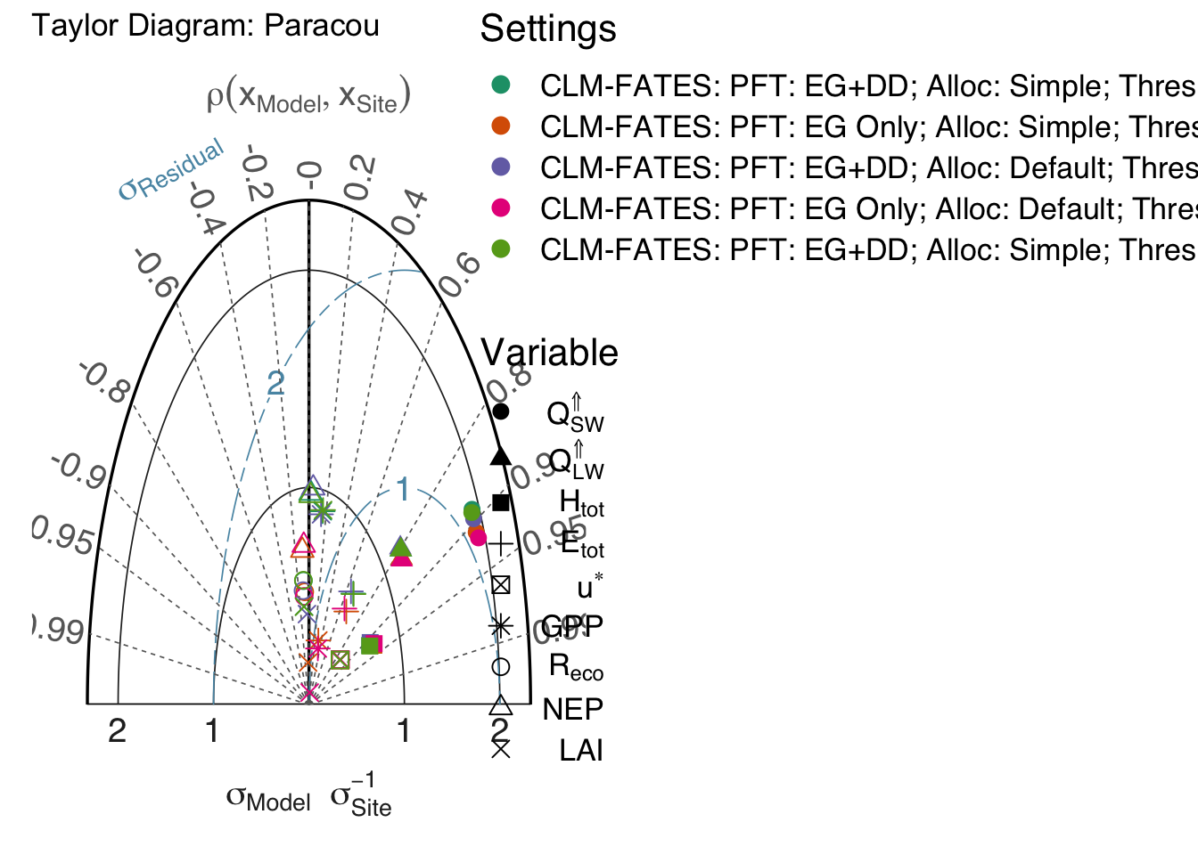
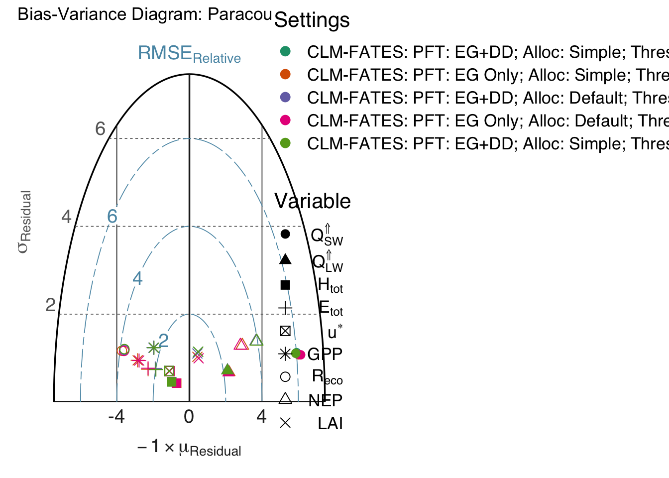
Generate the bias-variance diagrams, accounting for all variables and separating by season. Multiple model runs can be also provided for model improvement assessment. This is done by function RUtils/gg_biasvar.r). The bias-variance diagram is inspired in the Taylor diagram, but instead of showing the correlation between reference and predictions, it focus on the properties of the residuals (by definition \(r = x_{\mathrm{obser}} - x_{\mathrm{model}}\)), specifically how bias (\(\mathrm{Bias}=-\mu_{r}\)) and standard deviation of the residuals contribute to the root mean square error (\(\mathrm{RMSE}\)).
Inputs
x. Data set (data.frame,data.table, ortibble), it can be coerced to tibble. It is often necessary to rearrange the data, check functionsdata.table::meltanddplyr::pivot_longerwhich may help.obser. Column inxthat represents the observations. Default is"obs". This column may contain multiple variables, sites, seasons, or other category, as long as they can be identified by another column inx.model. Column(s) inxthat represents the model results. Default is a single column named"mod". Each row should correspond to the equivalent value inobser.group. Column inxthat describes how to classify the data. Each group will have a specific colour in the diagram. If none is provided, a single point will be pooled.panel. Column inxthat describes how to split the data. Each panel will be plot in a separate sub-figure in the diagram. If none is provided, a single panel will be plot.model_optsandgroup_opts. List of options for handling model/group annotation in the legend (used only if more than one model/group exists):title. Title for legend caption.label. Labels for models or groups. In the case of model_opts, this must have the same length as variable model. In the case of group_opts, this must match the number of unique groups. Iflabelis not provided, the code will use the same category names as variable model. If variablegroupis a character, we strongly recomend to use a named vector in which the names match the values in the group column (e.g.group_label = c(class_a = "A", class_b = "B").
colour_opts. List of options for colours. The following elements can be provided:by. In case multiple models and groups are provided, usebyto indicate which dimension should be distinguished by colour. Options are"model"or"group". The other one will be distinguished by shape. In case only one of them have multiple categories, we ignorebyand use both shape and colours to distinguish the categories.level. Colours for the categories distinguished by shapes. IfNULL, the colours will be automatically assigned. Otherwise, this can be a palette from packageRColorBrewer, a palette in packageviridis, a function that takes the number of sought colours as the first argument, or a vector with as many colours as categories.reverse. In case colour is a palette or function, reverse it?
shape_opts. List of options for shapes. The following elements can be provided:level. List of shapes for the categories distinguished by shapes. It can be a vector of numbers (same as those defined by lty) or characters (similar toggplot), with as many elements as categories. IfNULL, the shapes will be automatically assigned. Important: avoid using many more than 6 shapes because it makes the plot difficult to read.solid. In case shape isNULL, use solid shapes (TRUE or FALSE).size. Size for symbols.
panel_opts. List with options for panels. The following elements can be provided:label. Labels, to appear in the sub-plot titles (used only if more than one panel exists). This must match the number of unique groups. If none is provided, the code will use the unique values in variable panel. If variable group is a character, we strongly recomend to use a named vector in which the names match the values in the panel column (e.g.label = c(class_a = "A", class_b = "B")).levels. Type of level to use for panel annotation tags. This follows the same idea ofpatchwork::plot_annotation. Options are"a"for lowercase letters,"A"for uppercase letters,"1"for numbers,"i"for lowercase Roman numerals,"I"for uppercase Roman numerals. Empty character will skip levels.prefix. String to appear before the tag.suffix. String to appear after the tag and before the panel labels.sep. Separator between tag, prefix, and suffix. There will be always a space between tag and labels if panel_levels is not empty.
axis_opts. List of options for the main axes.colour. Colour for main axes.linetype. Line type for main axes.size. Line width for main axes.
bias_opts,sigma_opts,rmse_opts`. List of options for the bias, standard deviation of residuals (sigma), and root mean square error (RMSE) “axes” and labels:name. Name for this “axis”.at. Labels for this axis. IfNULLthis will be automatically defined.colour. Colour for this axis and labels.linetype. Line type for this axis.size. Line width for this axis.family. Font family for axis and labels.fontsize. Font size for axis and labels.
main_title. General title for the entire figure (single title even for multiple panels).extra_legend. Add extra plot space for legend?TRUEmeans yes,FALSE(default) means no.show_nsme. Replace the \(\sigma\) axis with the Nash-Sutcliffe model efficiency index?TRUEmeans yes,FALSE(default) means no. If this is TRUE, the values of sigma_opts$at will be overwritten.base_size. Size for theme.base_family. Family of font type for theme.
Output
This function returns a patchwork structure (compatible with ggplot).
# Temporary, load function
source(file.path(util_path,"gg_biasvar.r"))

if (n_case_info == 1){
   # Select data
   td_eval         = td_season
   td_title        = "Season"
   td_model        = c("DJF","MAM","JJA","SON")
   td_label        = c(DJF="DJF",MAM="MAM",JJA="JJA",SON="SON")
}else{
   td_eval         = td_config
   td_model        = case_info$name
   td_title        = "Settings"
   td_label        = paste0(case_info$model,": ",case_info$desc)
   names(td_label) = case_info$name
}#end if (n_case_info == 1)


# Set labels for variables
group_label        = hlm1dvar$short[match(var_both,hlm1dvar$vnam)]
names(group_label) = var_both
group_label        = mapply(FUN=parse,text=as.list(group_label))

# Generate bias-variance diagrams (one per season).
gg_good = gg_biasvar( x                  = td_eval
                    , obser              = "site"
                    , model              = td_model
                    , group              = "variable"
                    , panel              = NULL # "season"
                    , model_opts         = list( title = td_title
                                               , label = td_label
                                               )#end list
                    , group_opts         = list( title = "Variable", label = group_label)
                    , colour_opts        = list(by="model")
                    , main_title         = paste0("Bias-Variance Diagram: ",case_pref)
                    , base_size          = gg_ptsz
                    , show_nsme          = FALSE
                    , extra_legend       = TRUE
                    )#end gg_taylor
# Save plots.
for (d in sequence(ndevice)){
   h_output = paste0("biasvar_diag-",case_pref,".",gg_device[d])
   dummy    = ggsave( filename = h_output
                    , plot     = gg_good
                    , device   = gg_device[d]
                    , path     = taylor_biasvar_path
                    , width    = gg_width
                    , height   = gg_height
                    , units    = gg_units
                    , dpi      = gg_depth
                    )#end ggsave

}#end for (d in sequence(ndevice))

# If sought, plot images on screen
if (gg_screen) gg_good