Main script
Note: Changes beyond this point are only needed if you are developing the notebook.
Initial settings
First, we load some useful packages and tools, using the R script
load.everything.r. This will load all the R scripts at the
util_path directory.
source(file.path(util_path,"load.everything.r"),chdir=TRUE)We then set some of the paths that will be used for the output files. Normally these paths should not be changed.
- case_path is the main directory where the simulations are located.
- simul_path is a vector with all the possible paths were ELM-FATES or CLM-FATES can be written.
- tsage_path is the path for time series separated by patch age classes.
- tsdbh_path is the path for time series separated by size (diameter at breast height or DBH) classes.
- tspft_path is the path for time series separated by plant functional type.
- tsmort_path is the path for time series of mortality separated by mortality type (and shown for each PFT and each size class).
- tsdap_path is the path for time series by size and dbh, shown as heat maps: y is the size class, variables shown as heat maps, each panel being a different PFT.
- tssoil_path is the path for time series for soil variables, with depth as the y axis and the variable as a heat map.
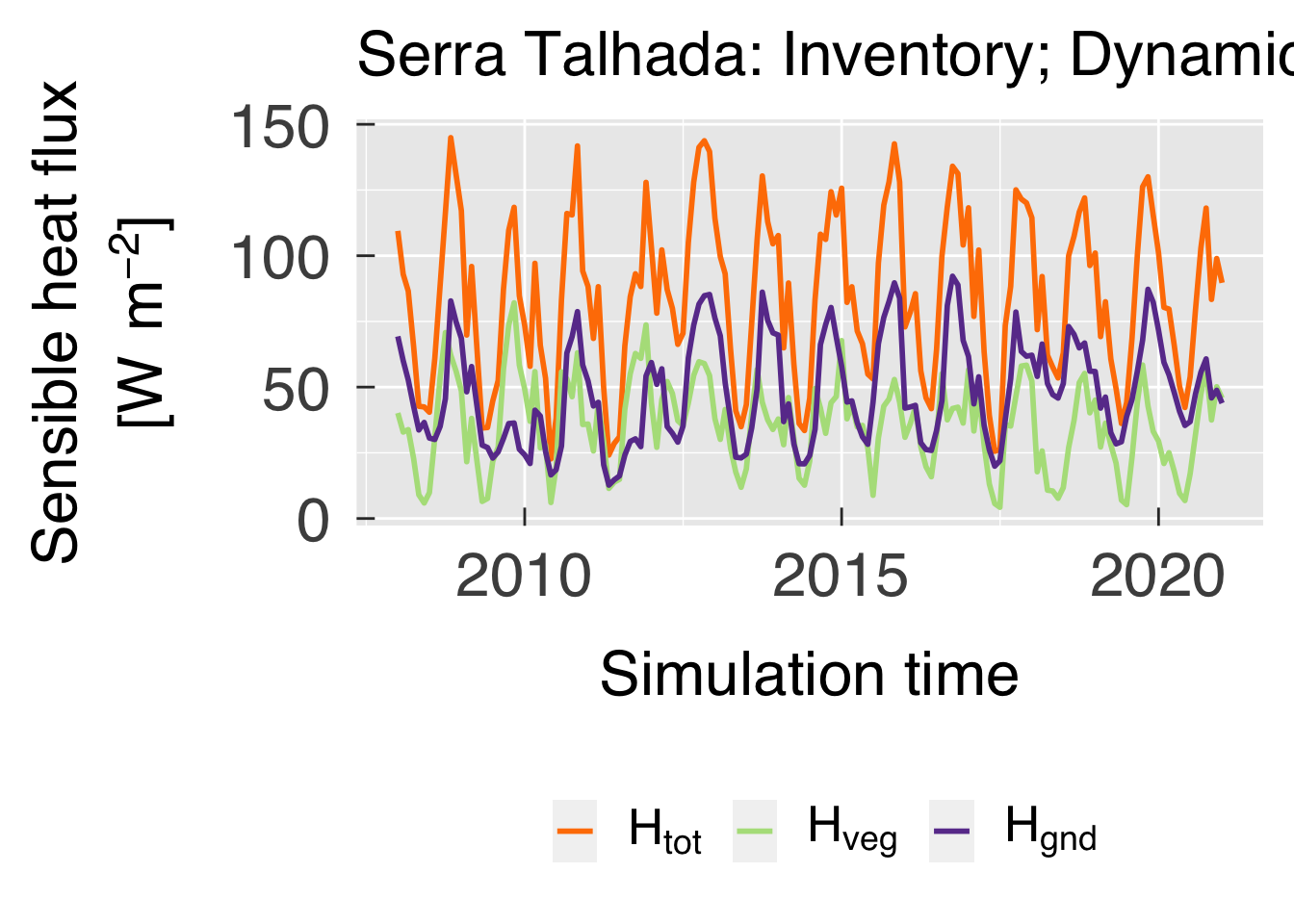
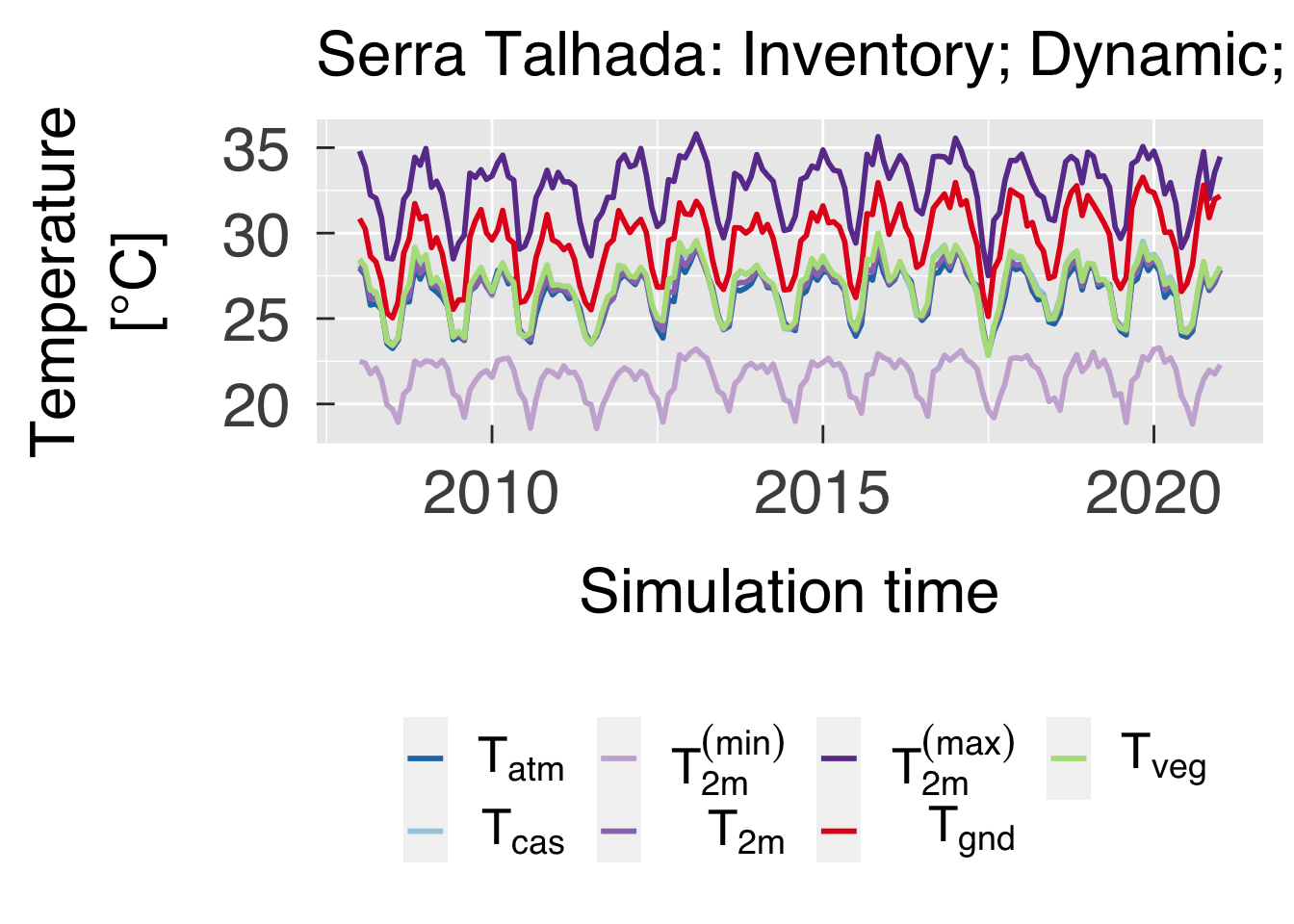
- tstheme_path is the path for time series with multiple variables, grouped under a common theme, such as energy fluxes or ecosystem productivity.
# Case path.  Do not change this unless you used non-standard case output for ELM/CLM.
case_path = file.path(hesm_main,case_fpref)

#---~---
#    Vector with all possible ELM/CLM paths containing NetCDF history files.  Do not change
# this unless you know what you are doing.
#---~---
simul_path = c( file.path(case_path,"run"), file.path(case_path,"lnd","hist"))

# Output path for time series
tsage_path    = file.path(plot_main,"tseries_age"         )
tsdbh_path    = file.path(plot_main,"tseries_dbh"         )
tspft_path    = file.path(plot_main,"tseries_pft"         )
tsmort_path   = file.path(plot_main,"tseries_mort"        )
tsalloc_path  = file.path(plot_main,"tseries_alloc_organ" )
tsauto_path   = file.path(plot_main,"tseries_auto_resp"   )
tsdap_path    = file.path(plot_main,"ts_heat_dbh+pft"     )
tsdphen_path  = file.path(plot_main,"ts_drought_phenology")
tssoil_path   = file.path(plot_main,"ts_heat_soil"        )
tstheme_path  = file.path(plot_main,"tseries_theme"       )

# Create paths for time series
dummy = dir.create(data_path   , recursive = TRUE, showWarnings = FALSE)
dummy = dir.create(tsage_path  , recursive = TRUE, showWarnings = FALSE)
dummy = dir.create(tsdbh_path  , recursive = TRUE, showWarnings = FALSE)
dummy = dir.create(tspft_path  , recursive = TRUE, showWarnings = FALSE)
dummy = dir.create(tsmort_path , recursive = TRUE, showWarnings = FALSE)
dummy = dir.create(tsalloc_path, recursive = TRUE, showWarnings = FALSE)
dummy = dir.create(tsauto_path , recursive = TRUE, showWarnings = FALSE)
dummy = dir.create(tsdap_path  , recursive = TRUE, showWarnings = FALSE)
dummy = dir.create(tsdphen_path, recursive = TRUE, showWarnings = FALSE)
dummy = dir.create(tssoil_path , recursive = TRUE, showWarnings = FALSE)
dummy = dir.create(tstheme_path, recursive = TRUE, showWarnings = FALSE)
Define the name of the file that will have the loaded variables in R-friendly format.
# Set the file name for output
rdata_base = paste0("Monthly_",case_name,".RData")
rdata_file = file.path(data_path,rdata_base)
We also list all colour palettes from packages
RColorBrewer and viridis. This will be useful
when deciding the colour ramps.
# List of palettes in package RColorBrewer and viridis
brewer_pal_info  = rownames(RColorBrewer::brewer.pal.info)
viridis_pal_info = as.character(lsf.str("package:viridis"))
viridis_pal_info = viridis_pal_info[! grepl(pattern="^scale_",x=viridis_pal_info)]
Next, we find the correct simulation path. We search for files in the
typical paths in which ELM-FATES or CLM-FATES simulations would be
located (simul_path). Once we find the correct path, we
update simul_path to the correct one. We also list all the
files and identify which one is the actual first history output from
FATES. The first file (full file name stored in variable
nc_zero) has additional information that can be useful, so
we must access the file even if it is not intended for output
analysis.
cat0(" + Search FATES output.")

hlm_midfix = c("elm.h0","clm2.h0")
nc_base    = paste0(case_fpref,".",hlm_midfix,"\\.....-..\\.nc")
nc_file    = file.path( rep(x = simul_path, times = length(nc_base   ))
                      , rep(x = nc_base   , each  = length(simul_path))
                      )#end file.path
nc_success = FALSE
for (d in seq_along(nc_file)){
   nc_path = dirname(nc_file[d])
   nc_base = basename(nc_file[d])
   nc_list = list.files(path=nc_path,pattern=nc_base)
   if (length(nc_list) > 0){
      # When finding the files, update nc_success find the first and last time.
      nc_success = TRUE

      # Find file name and the length of each file
      nc_nfile = length(nc_list)
      nc_nchar = nchar(nc_list[1])

      # Find all times
      nc_year   = as.numeric(substring(nc_list,nc_nchar-9,nc_nchar-6))
      nc_month  = as.numeric(substring(nc_list,nc_nchar-4,nc_nchar-3))
      nc_tstamp = make_datetime(year=nc_year,month=nc_month)

      # Find the first and last time available.
      i1st       = which.min(nc_tstamp)
      ilst       = which.max(nc_tstamp)
      nc_t1st    = nc_tstamp[i1st]
      nc_tlst    = nc_tstamp[ilst]
      tstamp_1st = sprintf("%2.2i/%2.2i/%4.4i",month(nc_t1st),day(nc_t1st),year(nc_t1st))
      tstamp_lst = sprintf("%2.2i/%2.2i/%4.4i",month(nc_tlst),day(nc_tlst),year(nc_tlst))

      # Save the path and "midfix" that worked.
      simul_path = nc_path
      nc_zero    = file.path(simul_path,nc_list[1])
      sel_midfix = mapply(FUN=grepl,pattern=as.list(hlm_midfix),MoreArgs=list(x=nc_base))
      hlm_midfix = hlm_midfix[sel_midfix]
   }#end if (length(nc_list) > 0)
}#end for (d in seq_along(nc_file))

# Do not continue if files were not found
if (! nc_success){
   stop(" Files were not found in any of the usual directories. Make sure basal paths are properly set.")
}#end if (! nc_success)
We set the times for which we will retrieve simulation results. A few noteworthy variables.
- tstamp0. First simulation time. This is always the actual first output file of the simulation, because the first output always has additional variables that are useful for analyses.
- tstampa. First time used for output. If
case_tstampawas set asNA_character_at the beginning of the script, we will use the first available time. - tstampz. Last time used for output. If
thiscase_tstampzwas set asNA_character_` at the beginning of the script, we will use the last available time. - tstamp. The vector with all times that should be loaded.
- ntstamp. The total count of time steps to load.
# Extract date information from string
if (! "tstamp0" %in% ls()){
   tstamp0 = as.integer(unlist(strsplit(tstamp_1st,split="/")))
   year0   = tstamp0[3]
   month0  = tstamp0[1]
}#end if (is.character(tstampa))
if (is.na(case_tstampa)){
   tstampa = as.integer(unlist(strsplit(tstamp_1st,split="/")))
   yeara   = tstampa[3]
   montha  = tstampa[1]
}else{
   tstampa = as.integer(unlist(strsplit(case_tstampa,split="/")))
   yeara   = tstampa[3]
   montha  = tstampa[1]
}#end if (is.character(tstampa))
if (is.na(case_tstampz)){
   tstampz = as.integer(unlist(strsplit(tstamp_lst,split="/")))
   yearz   = tstampz[3]
   monthz  = tstampz[1]
}else{
   tstampz = as.integer(unlist(strsplit(case_tstampz,split="/")))
   yearz   = tstampz[3]
   monthz  = tstampz[1]
}#end if (is.character(tstampz))

# Useful variables to build time stamps.
nmontha   = 12 - montha + 1          # Number of months in yeara
nmidyears = max(0,yearz - yeara - 1) # Number of years in between yeara and yearz
nmonthz   = monthz                   # Number of months in yearz

# Create lubridate object for initial and final time
tstampa = make_datetime( year=yeara,month=montha,day=1L)
tstampz = make_datetime( year=yearz,month=monthz,day=1L)

# Create month and year vector
if (yeara == yearz){
   # Simulation did not last more than one year
   tmonth = seq(from=montha,to=monthz,by=1)
   tyear  = rep(x=yeara,times=length(tmonth))
}else{
   # Simulation lasted longer than a year.
   tmonth = c( seq(from=montha,to=12,by=1)
             , rep(sequence(12),times=nmidyears)
             , seq(from=1     ,to=monthz,by=1)
             )#end c
   tyear  = c( rep(yeara,each=nmontha)
             , rep(yeara+sequence(nmidyears),each=12)
             , rep(yearz,each=nmonthz)
             )#end c
}#end if (yeara == yearz)

# Create time stamp and find how many times should be processed.
tstamp = make_datetime(year=tyear,month=tmonth,day=1L)
ntstamp = length(tstamp)
Decide which files to load. This is done because if the script is loading the files on the fly, this avoids trying to read a file that is just being created, which causes R to crash.
cat0(" + Run a file inventory to decide which files to load.")

nc_schedule = tibble( month = lubridate::month(tstamp)
                    , year  = lubridate::year (tstamp)
                    , ymlab = sprintf("%4.4i-%2.2i",year,month)
                    , base  = paste0(case_fpref,".",hlm_midfix,"." ,ymlab,".nc")
                    , file  = file.path(simul_path,base)
                    , load  = file.exists(file)
                    )#end tibble

# Simplify tibble
nc_schedule = nc_schedule %>% select(! ymlab)

# Find the last time that can be loaded
ntstamp_last = max(which(nc_schedule$load))
Before we proceed, we load the very first output file (at time
tstamp0, file nc_zero), to retrieve
information on dimensions, soil settings, indices to map the size and
PFT classes in some variables. We also compare the variables available
in nc_zero with those defined in variables
fatesvar (file
<util_path>/fates_varlist.r) and
hlm1dvar (file
<util_path>/hlm1d_varlist.r). We then create data
place holders for variables that are requested and available. We will
save legend information for the following dimensions (table elements are
the variable names):
| Dimension | Values | Element count | Keys (dimnames) |
Labels for axes |
|---|---|---|---|---|
| Patch age | ages |
nages |
agekeys |
agelabs |
| Size (DBH) | dbhs |
ndbhs |
dbhkeys |
dbhlabs |
| PFT | pftinfo$id |
npfts |
pftinfo$key |
pft$short |
We also create the following lists containing multiple arrays with data. We will later convert them into tibbles.
- byage. List of variables aggregated by patch age class.
- bydbh. List of variables aggregated by cohort size (DBH) classes.
- bypft. List of variables aggregated by plant functional type (PFT).
- hlm1d. List of scalar variables, many of handled by the host land model.
if ("nc_conn" %in% ls()){dummy = nc_close(nc_conn); rm(nc_conn)}

if (reload_rdata && file.exists(rdata_file)){
   # Load the previous data session.
   cat0(" + Load the data from previous sessions (",rdata_base,").")
   dummy = load(rdata_file)
}else{
   # We always read the first actual simulation time because it has more information.
   # Open NetCDF connection and retrieve variable names
   nc_conn  = nc_open(filename=nc_zero)
   nc_nvars = nc_conn$nvars
   nc_ndims = nc_conn$ndims
   nc_dlist = rep(NA_character_,times=nc_ndims)
   nc_vlist = rep(NA_character_,times=nc_nvars)
   for (d in sequence(nc_ndims)) nc_dlist[d] = nc_conn$dim[[d]]$name
   for (v in sequence(nc_nvars)) nc_vlist[v] = nc_conn$var[[v]]$name

   #---~---
   # Gather dimension information, then initialise matrices
   #---~---

   # List of age classes
   idxage   = match("fates_levage",nc_dlist)
   if (is.finite(idxage)){
      ages     = nc_conn$dim[[idxage]]$vals
      nages    = nc_conn$dim[[idxage]]$len

      ageinfo  = tibble( id      = sequence(nages)
                       , age_lwr = ages
                       , age_upr = c(ages[-1],Inf)
                       , key     = sprintf("age_%3.3i",ages)
                       , desc    = c( paste0("paste(paste(",age_lwr[-nages],"<= A*g*e)<",age_upr[-nages],"*y*r)")
                                    , paste0("paste( A*g*e >=",age_upr[nages],"*y*r)")
                                    )#end c
                       , labs    = c( paste0("paste(",age_lwr[-nages],"-",age_upr[-nages],")")
                                    , paste0("paste(",age_lwr[ nages],"-infinity)")
                                    )#end c
                       , colour  = viridis(nages,option="D",direction=-1)
                       )#end tibble
   }else{
      ageinfo  = tibble( id      = integer(0L)
                       , age_lwr = numeric(0L)
                       , age_upr = numeric(0L)
                       , key     = character(0L)
                       , desc    = character(0L)
                       , labs    = character(0L)
                       , colour  = character(0L)
                       )#end tibble
   }#end if (is.na(idxage))

   # Set number of age classes
   nages = nrow(ageinfo)


   # List of size classes
   idxdbh   = match("fates_levscls",nc_dlist)
   if (is.finite(idxdbh)){
      dbhs     = nc_conn$dim[[idxdbh]]$vals
      ndbhs    = nc_conn$dim[[idxdbh]]$len
      dbhinfo  = tibble( id      = sequence(ndbhs)
                       , dbh_lwr = dbhs
                       , dbh_upr = c(dbh_lwr[-1],dbh_lwr[ndbhs]+2*max(diff(dbh_lwr)))
                       , dbh     = 0.5 * (dbh_lwr + dbh_upr)
                       , key     = sprintf("dbh_%3.3i",dbh_lwr)
                       , desc    = c( paste0("paste(paste(",dbh_lwr[-ndbhs],"<=D*B*H)<",dbh_upr[-ndbhs],"*c*m)")
                                    , paste0("paste( D*B*H >=",dbh_lwr[ndbhs],"*c*m)")
                                    )#end c
                       , labs    = c( paste0("paste(",dbh_lwr[-ndbhs],"-",dbh_upr[-ndbhs],")")
                                    , paste0("paste(",dbh_lwr[ ndbhs],"-infinity)")
                                    )#end dbhlabs
                       , colour   = magma(ndbhs+1L,direction=1)[sequence(ndbhs)]
                       )#end tibble
   }else{
      dbhinfo  = tibble( id      = integer(0L)
                       , dbh_lwr = numeric(0L)
                       , dbh_upr = numeric(0L)
                       , key     = character(0L)
                       , desc    = character(0L)
                       , labs    = character(0L)
                       , colour  = character(0L)
                       )#end tibble
   }#end if (is.finite(idxdbh))

   # Set number of size classes
   ndbhs = nrow(dbhinfo)

   # List of PFT classes (only if not using user-defined classes).
   idxpft   = match("fates_levpft",nc_dlist)
   if (! is.finite(idxpft)){
      # PFT index not found. Skip PFTs altogether.
      pftinfo = tibble( id               = numeric(0L)
                      , key              = character(0L)
                      , short            = character(0L)
                      , desc             = character(0L)
                      , parse            = character(0L)
                      , colour           = character(0L)
                      )#end data.table
   }else if (! user_pftinfo){
      # Select all PFTs available
      pftids  = nc_conn$dim[[idxpft]]$vals
      npftids = nc_conn$dim[[idxpft]]$len

      # Build tibble with all the PFTs.
      pftinfo = tibble( id               = pftids
                      , key              = sprintf("pft%2.2i" ,pftids)
                      , short            = sprintf("PFT%2.2i" ,pftids)
                      , desc             = sprintf("PFT %2.2i",pftids)
                      , parse            = paste0("P*F*T*phantom(1)*",sprintf("%2.2i",pftids))
                      , colour           = brewer.pal(n=npftids,name="PuBuGn")
                      )#end tibble
   }#end if (! is.finite(idxpft))

   # Set number of PFTs (active PFTs only)
   npfts = nrow(pftinfo)


   # Load soil layers
   slayer = tibble( zsoi   = rev(c(unlist(ncvar_get(nc=nc_conn,varid="ZSOI"  ))))
                  , dzsoi  = rev(c(unlist(ncvar_get(nc=nc_conn,varid="DZSOI" ))))
                  , bsw    = rev(c(unlist(ncvar_get(nc=nc_conn,varid="BSW"   ))))
                  , hksat  = rev(c(unlist(ncvar_get(nc=nc_conn,varid="HKSAT" ))))
                  , sucsat = rev(c(unlist(ncvar_get(nc=nc_conn,varid="SUCSAT"))))
                  , watsat = rev(c(unlist(ncvar_get(nc=nc_conn,varid="WATSAT"))))
                  )#end data.table

   # Set number of soil layers
   nslzs   = nrow(slayer)


   # Find the deepest level to be considered (shallowest bedrock layer)
   n_bedrock = nslzs - ncvar_get(nc=nc_conn,varid="nbedrock") + 1


   # List of soil level classes
   slzinfo = tibble( id      = sequence(nslzs)
                   , key     = sprintf("slz_%4.4i",round(100.*slayer$zsoi))
                   , slz     = - slayer$zsoi
                   , slz_lwr = - rev(cumsum(rev(slayer$dzsoi)))
                   , slz_upr = c(slz_lwr[-1],0.5*slz[nslzs])
                   , desc    = paste0("paste(paste(",sprintf("%.3g",abs(slz_upr)),"<= z)<"
                                                    ,sprintf("%.3g",abs(slz_lwr)),"*m)")
                   , labs    = paste0("paste(",sprintf("%.3g",abs(slz_upr))
                                          ,"-",sprintf("%.3g",abs(slz_lwr)),")")
                   , show   = TRUE
                   , colour = "transparent"
                   )#end tibble

   # Define which soil layers to show, and assign colours (keep invalid layers transparent)
   slz_show     = max(slz_deepest,slzinfo$slz[n_bedrock])
   slzinfo      = slzinfo %>% mutate( show = slz_upr > slz_show )
   nslzs_show   = sum(slzinfo$show)
   slzinfo$colour[slzinfo$show] = cividis(n=nslzs_show,direction=-1)

   # Retrieve all variables by age class.
   nc_byage = nc_vlist[grepl(pattern="_AP$",x=nc_vlist)]
   nc_pref  = tolower(gsub(pattern="_AP$",replacement="",x=nc_byage))
   nc_keep  = nc_pref %in% fatesvar$vnam & (! duplicated(nc_pref))
   no_byage = nc_byage[! nc_keep]
   nc_byage = nc_byage[  nc_keep]
   nbyage   = length(nc_byage)


   #---~---
   #    Retrieve all variables by size class. We also test for variables that can be
   # obtained from adding under storey and canopy.
   #---~---
   is_size     = grepl(pattern="_SZ$",x=nc_vlist) | grepl(pattern="_SZPF$",x=nc_vlist)
   nc_bydbh    = nc_vlist[is_size]
   nc_pref     = gsub(pattern="_SZ$",replacement="",x=nc_bydbh)
   nc_pref     = gsub(pattern="_SZPF$",replacement="",x=nc_pref )
   nc_pref     = tolower(nc_pref)
   nc_keep     = (nc_pref %in% fatesvar$vnam) & (! duplicated(nc_pref))
   no_bydbh    = nc_bydbh[! nc_keep]
   nc_bydbh    = unique(nc_bydbh[  nc_keep])
   vardbh_last = rep(x=FALSE,times=nfatesvar)
   for (v in which(fatesvar$is_upc)){
      nc_vnow      = toupper(fatesvar$vnam[v])
      nc_vnow_size = paste0(nc_vnow,"_SZ")
      nc_vund_size = paste0(nc_vnow,"_USTORY_SZ")
      nc_vcan_size = paste0(nc_vnow,"_CANOPY_SZ")
      nc_vnow_szpf = paste0(nc_vnow,"_SZPF")
      nc_vund_szpf = paste0(nc_vnow,"_USTORY_SZPF")
      nc_vcan_szpf = paste0(nc_vnow,"_CANOPY_SZPF")

      # Check whether this variable can be derived from understorey+canopy (and needs to be).
      if ( all(c(nc_vund_size,nc_vcan_size) %in% nc_bydbh ) && (! nc_vnow_size %in% nc_bydbh) ){
         nc_bydbh       = unique(c(nc_bydbh,nc_vnow_size))
         vardbh_last[v] = TRUE
      }else if ( all(c(nc_vund_szpf,nc_vcan_szpf) %in% nc_bydbh ) && (! nc_vnow_szpf %in% nc_bydbh) ){
         nc_bydbh       = unique(c(nc_bydbh,nc_vnow_szpf))
         vardbh_last[v] = TRUE
      }#end if ( all(c(nc_vund_size,nc_vcan_size) %in% nc_bydbh ) && (! nc_vnow_size %in% nc_bydbh) )
   }#end for (v in which(fatesvar$is_upc))

   # In case both size and size+PFT values were given for the same vaariable, remove the size-only one.
   nc_ancil      = sort(gsub(pattern="_SZ$",replacement="_SZZZ",x=nc_bydbh))
   nc_ancil      = gsub(pattern="_SZZZ$",replacement="_SZPF",nc_ancil)
   nc_duplicated = nc_ancil[duplicated(nc_ancil)]
   nc_bydbh      = nc_bydbh[! (nc_bydbh %in% nc_duplicated)]

   # Tally the total number of DBH variables, and derived variables.
   nbydbh        = length(nc_bydbh)
   n_vardbh_last = sum(vardbh_last)


   #---~---
   #    Retrieve all variables by PFT. We also test for variables that can be
   # obtained from adding under storey and canopy.
   #---~---
   is_pft      = grepl(pattern="_SZPF$",x=nc_vlist)
   nc_bypft    = nc_vlist[is_pft]
   nc_pref     = tolower(gsub(pattern="_SZPF$",replacement="",x=nc_bypft ))
   nc_keep     = nc_pref %in% fatesvar$vnam & (! duplicated(nc_pref))
   no_bypft    = nc_bypft[! nc_keep]
   nc_bypft    = unique(nc_bypft[  nc_keep])
   varpft_last = rep(x=FALSE,times=nfatesvar)
   for (v in which(fatesvar$is_upc)){
      nc_vnow      = toupper(fatesvar$vnam[v])
      nc_vnow_szpf = paste0(nc_vnow,"_SZPF")
      nc_vund_szpf = paste0(nc_vnow,"_USTORY_SZPF")
      nc_vcan_szpf = paste0(nc_vnow,"_CANOPY_SZPF")

      # Check whether this variable can be derived from understorey+canopy (and needs to be).
      if ( all( c(nc_vund_szpf,nc_vcan_szpf) %in% nc_bypft ) && (! nc_vnow_szpf %in% nc_bypft) ){
         nc_bypft       = unique(c(nc_bypft,nc_vnow_szpf))
         varpft_last[v] = TRUE
      }#end if ( all(c(nc_vund_size,nc_vcan_size) %in% nc_bydbh ) && (! nc_vnow_size %in% nc_bydbh) )
   }#end for (v in which(fatesvar$is_upc))

   # Tally the total number of PFT variables, and derived variables.
   nbypft    = length(nc_bypft)
   n_varpft_last = sum(varpft_last)


   #---~---
   #    Retrieve all "drought deciduous phenology variables
   #---~---
   nc_pref   = tolower(x=nc_vlist)
   nc_keep   = nc_pref %in% dphenvar$vorig
   no_dphen  = nc_vlist[! nc_keep]
   nc_dphen  = nc_vlist[  nc_keep]

   # Tally the total number of drought phenology variables.
   ndphen = length(nc_dphen)


   #---~---
   #    Retrieve all "1D" variables that are available at the host model.
   #---~---
   nc_pref   = tolower(x=nc_vlist)
   nc_keep   = nc_pref %in% hlm1dvar$vnam
   no_hlm1d  = nc_vlist[! nc_keep]
   nc_hlm1d  = nc_vlist[  nc_keep]

   # Check whether to append "evapotranspiration"
   if (  ( all(c("QSOIL","QVEGT","QVEGE") %in% nc_hlm1d) ) && (! "QEVTR" %in% nc_hlm1d) ){
      nc_hlm1d = unique(c(nc_hlm1d,"QEVTR"))
      etr_last = TRUE
   }else{
      etr_last = FALSE
   }#end if (  ( all(c("QSOIL","QVEGT","QVEGE") %in% nc_hlm1d) ) && (! "QEVTR" %in% nc_hlm1d) )

   # Check whether to append ecosystem respiration (HLM)
   if (  ( all(c("AR","HR") %in% nc_hlm1d) ) && (! "ER" %in% nc_hlm1d) ){
      nc_hlm1d = unique(c(nc_hlm1d,"ER"))
      er_last  = TRUE
   }else{
      er_last  = FALSE
   }#end if (  ( all(c("AR","HR") %in% nc_hlm1d) ) && (! "ER" %in% nc_hlm1d) )

   # Check whether to append ecosystem respiration (FATES)
   if (  ( all(c("FATES_AUTORESP","FATES_HET_RESP") %in% nc_hlm1d) ) && (! "FATES_ECORESP" %in% nc_hlm1d) ){
      nc_hlm1d = unique(c(nc_hlm1d,"FATES_ECORESP"))
      fates_er_last  = TRUE
   }else{
      fates_er_last  = FALSE
   }#end if (  ( all(c("AR","HR") %in% nc_hlm1d) ) && (! "ER" %in% nc_hlm1d) )

   # Find number of host land model variables
   nhlm1d    = length(nc_hlm1d)


   # Retrieve all "2D" soil variables that are available at the host model.
   nc_pref   = tolower(x=nc_vlist)
   nc_keep   = nc_pref %in% hlm2dsoi$vnam
   no_soi2d  = nc_vlist[! nc_keep]
   nc_soi2d  = nc_vlist[  nc_keep]

   # Find number of soil variables
   nsoi2d    = length(nc_soi2d)


   # Initialise list of variables by age class.
   byage  = list()
   for (a in sequence(nbyage)){
      nc_nvnow        = nc_byage[a]
      nc_pref         = tolower(gsub(pattern="_AP$",replacement="",x=nc_nvnow))
      f               = match(nc_pref,fatesvar$vnam)
      f_vnam          = fatesvar$vnam[f]
      byage[[f_vnam]] = matrix(data=NA_real_,nrow=ntstamp,ncol=nages,dimnames=list(NULL,ageinfo$key))
   }#end for (a in sequence(nbyage))


   # Initialise list of variables by size class
   bydbh = list()
   for (d in sequence(nbydbh)){
      nc_nvnow        = nc_bydbh[d]
      nc_pref         = gsub(pattern="_SZ$"  ,replacement="",x=nc_nvnow)
      nc_pref         = gsub(pattern="_SZPF$",replacement="",x=nc_pref )
      nc_pref         = tolower(nc_pref)
      f               = match(nc_pref,fatesvar$vnam)
      f_vnam          = fatesvar$vnam[f]
      bydbh[[f_vnam]] = matrix(data=NA_real_,nrow=ntstamp,ncol=ndbhs,dimnames=list(NULL,dbhinfo$key))
   }#end for (d in sequence(nbydbh))


   # Initialise list of variables by PFT class and by PFT and size class.
   bypft = list()
   bydap = list()
   for (p in sequence(nbypft)){
      nc_nvnow        = nc_bypft[p]
      nc_pref         = tolower(gsub(pattern="_SZPF$",replacement="",x=nc_nvnow))
      nc_pref         = tolower(nc_pref)
      f               = match(nc_pref,fatesvar$vnam)
      f_vnam          = fatesvar$vnam[f]
      bypft[[f_vnam]] = matrix( data     = NA_real_
                              , nrow     = ntstamp
                              , ncol     = npfts
                              , dimnames = list(NULL,pftinfo$key)
                              )#end matrix
      bydap[[f_vnam]] = array ( data     = NA_real_
                              , dim      = c(ntstamp,ndbhs,npfts)
                              , dimnames = list(NULL,dbhinfo$key,pftinfo$key)
                              )#end array
   }#end for (d in sequence(nbypft))


   # Initialise list of variables by soil layer
   dphen = list()
   for (p in sequence(ndphen)){
      nc_nvnow        = nc_dphen[p]
      nc_pref         = tolower(nc_nvnow)
      f               = match(nc_pref,dphenvar$vorig)
      f_vnam          = dphenvar$vnam[f]
      dphen[[f_vnam]] = matrix(data=NA_real_,nrow=ntstamp,ncol=npfts,dimnames=list(NULL,pftinfo$key))
   }#end for (p in sequence(ndphen))


   # Initialise 1D variables available at the HLM
   hlm1d = as_tibble( matrix( data     = NA_real_
                            , nrow     = ntstamp
                            , ncol     = nhlm1d
                            , dimnames = list(NULL,tolower(nc_hlm1d))
                            )#end matrix
                    )#end as.data.table


   # Initialise list of variables by soil layer
   soi2d = list()
   for (s in sequence(nsoi2d)){
      nc_nvnow        = nc_soi2d[s]
      nc_pref         = tolower(nc_nvnow)
      f               = match(nc_pref,hlm2dsoi$vnam)
      f_vnam          = hlm2dsoi$vnam[f]
      soi2d[[f_vnam]] = matrix(data=NA_real_,nrow=ntstamp,ncol=nslzs,dimnames=list(NULL,slzinfo$key))
   }#end for (s in sequence(nsoi2d))


   # Load indices. For PFTs, we keep both the original index (opft) and the remapped one (ipft).
   # We also save the order for loading the data, so they are aligned with the output indices.
   index_szpf = tibble( size   = ncvar_get(nc=nc_conn,varid='fates_scmap_levscpf'  )
                      , opft   = ncvar_get(nc=nc_conn,varid='fates_pftmap_levscpf' )
                      , ipft   = pftinfo$id[match(opft,pftinfo$od)]
                      , order  = order(ipft,size)
                      )#end data.table

   # Close connection
   dummy   = nc_close(nc_conn)
}#end if (reload_rdata && file.exists(rdata_file))
We then loop through the times to be read, and populate the place holders with the actual data sets. Most data sets should be available through the netCDF files, often with one of the following extensions.
- *_AP*. Variables that are aggregated by the patch age classes. These
are used for populating the
byagevariable structure. - *_SZ*. Variables that are aggregated by size. These are used for
populating the
bydbhvariable structure. - *_SZPF*. Variables that are aggregated by size and
plant functional type. These are used for populating the
bydbh,bypft, andbydapvariable structures.
Note. The extensions must be
suppressed when listing the variables in fatesvar in file
<util_path>/fates_varlist.r. Also, scalar variables
do not have unique extensions, so the full variable name must be
provided in hlm1dvar. The model
Besides variables that exist in the FATES output files, the following
variables can be set in <util_path>/fates_varlist.r
(for FATES variables that are aggregated by size, PFT, or age class) or
<util_path>/hlm_varlist.r (for variables mostly
associated with the host land model, 1-D FATES variables, or soil
variables). A few derived quantities are also allowed. * Any quantity
that has a “canopy” and “ustory” variable in FATES output, but no
variable that combines both readily available from the FATES history
files. In this case, both the “canopy” and “ustory” variables must be
listed in <util_path>/fates_varlist.r, as well as the
intended variable that combines both: this additional variable must have
the same prefix as the “canopy” and “ustory” variables (e.g., if
understory variable is lai_ustory and the canopy variable
is lai_canopy, the combined variable must be named
lai) and the is_upc flag for the combined variable in
<util_path>/fates_varlist.r must be set to
TRUE. * er (total ecosystem respiration) in
hlm1d_varlist, which will be available provided that
ar (autotrophic respiration) and hr (heterotrophic
respiration) are available too and defined in
hlm1d_varlist. * qevtr (total evaporation sensu Miralles et al.
2020 ) in hlm1d_varlist, which will be available
provided that qvege (evaporation from leaf surface water),
qvegt (transpiration) and qsoil (soil evaporation) are
available too and defined in hlm1d_varlist.
if (reload_rdata && file.exists(rdata_file)){
   ntstamp_first = w_resume
}else if (ntstamp_last > 0L){
   ntstamp_first = 1L
}else{
   # This can happen when files exist but they are outside the range for plotting.
   # Stop the run here.
   stop(" + No file to be loaded at this time, skip plotting.")
}#end if (reload_rdata && file.exists(rdata_file))

# Set loop
n_loop = max(0L,ntstamp_last - ntstamp_first + 1L)
if (n_loop > 0L){
   cat0(" + Load FATES results from time step ",ntstamp_first,".")
   w_loop  = seq(from=ntstamp_first,to=ntstamp_last,by=1L)
   ProgBar = txtProgressBar(max=n_loop,char=".",style=3L)
}else{
   cat0(" + No new data to be loaded this time.")
   w_loop = sequence(0L)
}#end (n_loop > 0L)

if ("nc_conn" %in% ls()){dummy = nc_close(nc_conn); rm(nc_conn)}
for (w in w_loop){
   # Extract times and build file name
   w_show   = w - ntstamp_first + 1L
   w_month  = nc_schedule$month[w]
   w_year   = nc_schedule$year [w]
   nc_base  = nc_schedule$base [w]
   nc_file  = nc_schedule$file [w]
   nc_show  = setTxtProgressBar(pb=ProgBar,value=w-w_show)


   # Find conversion factors for monthly variables.
   cmon.day = days_in_month(tstamp[w])
   cmon.hr  = day.hr  * cmon.day
   cmon.min = day.min * cmon.day
   cmon.sec = day.sec * cmon.day


   # Open NetCDF connection and retrieve variable names
   nc_conn  = nc_open(filename=nc_file)
   nc_nvars = nc_conn$nvars
   nc_vlist = rep(NA_character_,times=nc_nvars)
   for (v in sequence(nc_nvars)) nc_vlist[v] = nc_conn$var[[v]]$name


   # Read variables by age, and assign current values to the matrix.
   for (a in sequence(nbyage)){
      nc_nvnow            = nc_byage[a]
      nc_pref             = tolower(gsub(pattern="_AP$",replacement="",x=nc_nvnow))
      f                   = match(nc_pref,fatesvar$vnam)
      f_vnam              = fatesvar$vnam[f]
      f_add0              = eval(parse(text=fatesvar$add0[f]))
      f_mult              = eval(parse(text=fatesvar$mult[f]))
      nc_dat              = ncvar_get(nc=nc_conn,varid=nc_nvnow)
      byage[[f_vnam]][w,] = f_add0 + f_mult * nc_dat
   }#end for (a in sequence(nbyage))

   #---~---
   #   Read variables by size, and assign current values to the matrix.  In case
   # derived variables are in the list and they are the last variables, we calculate
   # them from canopy and understorey, after loading all other variables.
   #---~---
   for (d in sequence(nbydbh-n_vardbh_last)){
      nc_nvnow            = nc_bydbh[d]
      is_szpf             = grepl(pattern="_SZPF$",x=nc_nvnow)
      nc_pref             = gsub(pattern="_SZ$"  ,replacement="",x=nc_nvnow)
      nc_pref             = gsub(pattern="_SZPF$",replacement="",x=nc_pref )
      nc_pref             = tolower(nc_pref)
      f                   = match(nc_pref,fatesvar$vnam)
      f_vnam              = fatesvar$vnam[f]
      f_add0              = eval(parse(text=fatesvar$add0[f]))
      f_mult              = eval(parse(text=fatesvar$mult[f]))
      f_aggr              = match.fun(fatesvar$aggr[f])
      nc_dat              = ncvar_get(nc=nc_conn,varid=nc_nvnow)
      nc_dat              = f_add0 + f_mult * nc_dat
      if (is_szpf){
         # Reorder data for output
         nc_dat = nc_dat[index_szpf$order]

         # Aggregate data by size class
         nc_aggr        = tapply( X     = nc_dat
                                , INDEX = index_szpf$size
                                , FUN   = f_aggr
                                , na.rm = TRUE
                                )#end tapply
         names(nc_aggr) = NULL
         bydbh[[f_vnam]][w,] = nc_aggr
      }else{
         # Variable is truly a size class.
         bydbh[[f_vnam]][w,] = nc_dat
      }#end if (is_szpf)
   }#end for (d in sequence(nbydbh-n_vardbh_last))

   # Loop through variables to be added last
   for (v in which(vardbh_last)){
      # Retrieve variable and build understory and canopy variables.
      v_vnam = fatesvar$vnam[v]
      v_vund = paste0(v_vnam,"_ustory")
      v_vcan = paste0(v_vnam,"_canopy")

      # Aggregate data
      bydbh[[v_vnam]][w,] = bydbh[[v_vund]][w,] + bydbh[[v_vcan]][w,]
   }#end for (v in which(vardbh_last))


   #---~---
   #   Read variables by PFT and by size class and PFT, and assign current values to the matrix.  In case of
   # derived variables in the list and they are the last variables, we calculate
   # them from canopy and understorey, after loading all other variables.
   #---~---
   for (p in sequence(nbypft-n_varpft_last)){
      # Load variable information
      nc_nvnow = nc_bypft[p]
      nc_pref  = tolower(gsub(pattern="_SZPF$",replacement="",x=nc_nvnow))
      f        = match(nc_pref,fatesvar$vnam)
      f_vnam   = fatesvar$vnam[f]
      f_add0   = eval(parse(text=fatesvar$add0[f]))
      f_mult   = eval(parse(text=fatesvar$mult[f]))
      f_aggr   = match.fun(fatesvar$aggr[f])
      f_dbh01  = fatesvar$dbh01[f]

      # Retrieve data.
      nc_dat   = ncvar_get(nc=nc_conn,varid=nc_nvnow)

      # Apply unit conversion factors
      nc_dat   = f_add0 + f_mult * nc_dat

      # Copy the results to the size and PFT array
      bydap[[f_vnam]][w,,] = nc_dat[index_szpf$order]

      # Decide whether or not to exclude the first DBH class for PFT aggregation.
      if (f_dbh01){
         seldbh = rep(TRUE,times=length(nc_dat))
      }else{
         seldbh = ! (index_szpf$size %in% c(1))
      }#end if (f_dbh01)

      # Aggregate data by size class
      nc_aggr        = tapply( X     = nc_dat[seldbh]
                             , INDEX = index_szpf$ipft[seldbh]
                             , FUN   = f_aggr
                             , na.rm = TRUE
                             )#end tapply
      names(nc_aggr) = NULL

      # Bring only the PFTs we are interested in.
      bypft[[f_vnam]][w,] = nc_aggr
   }#end for (d in sequence(nbydbh-n_varpft_last))


   # Loop through variables to be added last
   for (v in which(varpft_last)){
      # Retrieve variable and build understory and canopy variables.
      v_vnam = fatesvar$vnam[v]
      v_vund = paste0(v_vnam,"_ustory")
      v_vcan = paste0(v_vnam,"_canopy")

      # Aggregate data
      bydap[[v_vnam]][w,,] = bydap[[v_vund]][w,,] + bydap[[v_vcan]][w,,]
      bypft[[v_vnam]][w, ] = bypft[[v_vund]][w, ] + bypft[[v_vcan]][w, ]
   }#end for (v in which(varpft_last))


   # Read drought-deciduous phenology variables (by PFT), and assign current values to the matrix.
   # We use "rev" because the first soil layer is the deepest for the R output.
   for (p in sequence(ndphen)){
      nc_nvnow            = nc_dphen[p]
      nc_pref             = tolower(nc_nvnow)
      f                   = match(nc_pref,dphenvar$vorig)
      f_vnam              = dphenvar$vnam[f]
      f_add0              = eval(parse(text=dphenvar$add0[f]))
      f_mult              = eval(parse(text=dphenvar$mult[f]))
      nc_dat              = ncvar_get(nc=nc_conn,varid=nc_nvnow)
      dphen[[f_vnam]][w,] = f_add0 + f_mult * rev(nc_dat)
   }#end for (a in sequence(nbyage))


   # Read 1D variables
   for (v in sequence(nhlm1d-etr_last-er_last-fates_er_last)){
      nc_nvnow            = nc_hlm1d[v]
      nc_pref             = tolower(x=nc_nvnow)
      h                   = match(nc_pref,hlm1dvar$vnam)
      h_vnam              = hlm1dvar$vnam[h]
      h_add0              = eval(parse(text=hlm1dvar$add0[h]))
      h_mult              = eval(parse(text=hlm1dvar$mult[h]))
      nc_dat              = ncvar_get(nc=nc_conn,varid=nc_nvnow)
      hlm1d[[h_vnam]][w]  = h_add0 + h_mult * nc_dat
   }#for (h in sequence(nhlm1d-etr_last-et_last))

   # Find total ET.
   if (etr_last){
      hlm1d$qevtr[w] = hlm1d$qvege[w] + hlm1d$qvegt[w] + hlm1d$qsoil[w]
   }#end if (etr_last)

   # Find total Ecosystem respiration (HLM)
   if (er_last){
      hlm1d$er[w] = hlm1d$ar[w] + hlm1d$hr[w]
   }#end if (er_last)

   # Find total Ecosystem respiration (FATES)
   if (fates_er_last){
      hlm1d$fates_ecoresp[w] = hlm1d$fates_autoresp[w] + hlm1d$fates_het_resp[w]
   }#end if (fates_er_last)


   # Read variables by soil layer, and assign current values to the matrix.
   # We use "rev" because the first soil layer is the deepest for the R output.
   for (s in sequence(nsoi2d)){
      nc_nvnow            = nc_soi2d[s]
      nc_pref             = tolower(nc_nvnow)
      f                   = match(nc_pref,hlm2dsoi$vnam)
      f_vnam              = hlm2dsoi$vnam[f]
      f_add0              = eval(parse(text=hlm2dsoi$add0[f]))
      f_mult              = eval(parse(text=hlm2dsoi$mult[f]))
      nc_dat              = ncvar_get(nc=nc_conn,varid=nc_nvnow)
      soi2d[[f_vnam]][w,] = f_add0 + f_mult * rev(nc_dat)
   }#end for (a in sequence(nbyage))


   # Close connection
   dummy    = nc_close(nc_conn)
}#end for (w in w_loop)
If any time was loaded, we save the current state. This allows for more efficient data loading for long runs.
# If any time was loaded, we save the new structures.
if (length(w_loop) > 0){
   w_resume = ntstamp_last + 1L

   # List of variables to be saved.
   save_list = c("ageinfo","nages","dbhinfo","ndbhs","pftinfo","npfts","slayer","nslzs"
                ,"n_bedrock","slzinfo","slz_show","nslzs_show","nc_byage","nbyage"
                ,"nc_bydbh","nbydbh","vardbh_last","n_vardbh_last","nc_bypft","nbypft"
                ,"nbypft","varpft_last","n_varpft_last","nc_dphen","ndphen","nc_hlm1d"
                ,"nhlm1d","etr_last","er_last","fates_er_last","nc_soi2d","nsoi2d","byage"
                ,"bydbh","bypft","bydap","dphen","hlm1d","soi2d","index_szpf","w_resume")

   # Save the current state of simulation
   cat0(" + Save data loaded so far to ",basename(rdata_base),".")
   dummy = save( list              = save_list
               , file              = rdata_file
               , compress          = "xz"
               , compression_level = 9
               )#end save
}#end if (length(w_loop) > 0)
Turn data matrices into molten tibble objects. These are compatible
with ggplot and are the preferred data structure for
analysing data efficiently using tidyverse. The variables
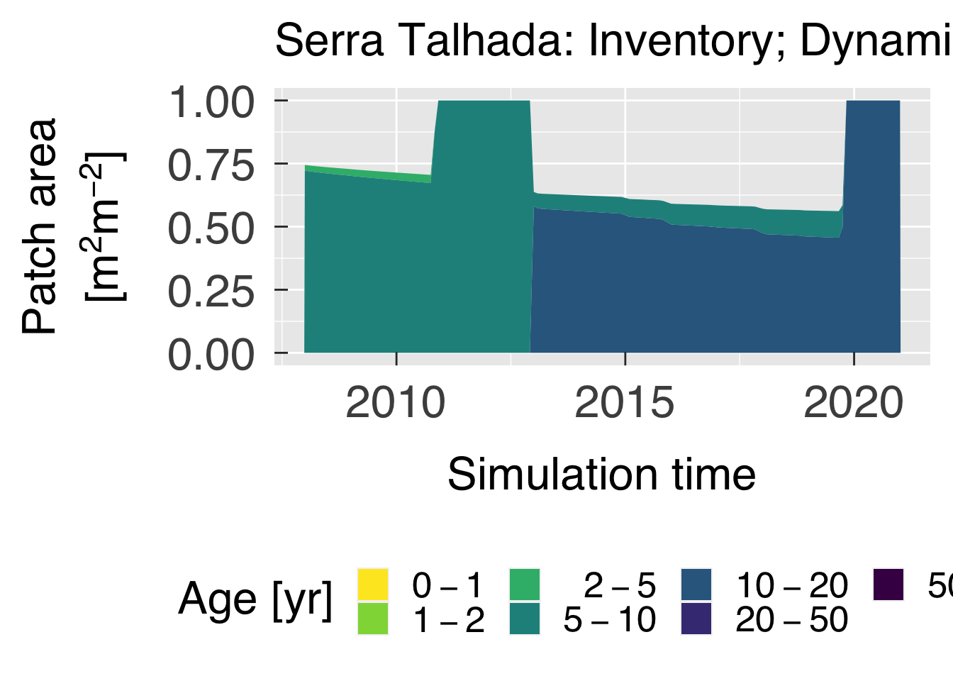
by age must also be scaled by patch area, and we do this in this block
too, to ensure this is not done more than once. Note that patch area by
age must be always included in FATES output. Patch area by age itself
should not be scaled.
# Turn age-dependent matrices into tibble objects
if (! is_tibble(byage)){
   cat0(" + Turn age-dependent matrices into tibble objects.")
   age_melt = NULL
   for (a in sequence(nbyage)){
      # Match variables.
      f        = match(names(byage)[a],fatesvar$vnam)
      f_vnam   = fatesvar$vnam[f]
      f_desc   = fatesvar$desc[f]
      f_stack  = fatesvar$stack[f]
      cat0("   - ",f_desc,".")

      # Check whether or not this variable needs to be scaled by area. Area itself should never be scaled.
      if (f_stack && (! (f_vnam %in% "patch_area"))){
         now_age = as_tibble(byage[[f_vnam]] * byage$fates_patcharea)
      }else{
         now_age = as_tibble(byage[[f_vnam]])
      }#end if (f_stack && (! (f_vnam %in% "patch_area")))

      # Create molten data table for this variable.
      now_age$time = tstamp
      now_melt     = as_tibble(melt(data=now_age,id.vars="time",variable.name="age",value.name=f_vnam))

      # Convert class to integer
      now_melt     = now_melt %>% mutate( age = as.integer(age))

      # Merge data table
      if (is.null(age_melt)){
         age_melt = now_melt
      }else{
         age_melt = as_tibble(merge(x=age_melt,y=now_melt,by=c("time","age"),all=TRUE))
      }#end if (is.null(age_melt))
   }#end for (a in sequence(nbyage))

   # Replace byage with the tibble object
   byage = age_melt
   rm(age_melt)
}#end if (! is_tibble(byage))


# Turn size-dependent matrices into data tables
if (! is_tibble(bydbh)){
   cat0(" + Turn size-dependent matrices into data tables.")
   dbh_melt = NULL
   for (d in sequence(nbydbh)){
      # Match variables.
      f        = match(names(bydbh)[d],fatesvar$vnam)
      f_vnam   = fatesvar$vnam[f]
      f_desc   = fatesvar$desc[f]
      cat0("   - ",f_desc,".")

      # Create molten data table for this variable.
      now_dbh      = as_tibble(bydbh[[d]])
      now_dbh$time = tstamp
      now_melt     = as_tibble(melt(data=now_dbh,id.vars="time",variable.name="dbh",value.name=f_vnam))

      # Convert class to integer
      now_melt     = now_melt %>% mutate( dbh = as.integer(dbh))

      # Merge data table
      if (is.null(dbh_melt)){
         dbh_melt = now_melt
      }else{
         dbh_melt = as_tibble(merge(x=dbh_melt,y=now_melt,by=c("time","dbh"),all=TRUE))
      }#end if (is.null(dbh_melt))
   }#end for (d in sequence(nbydbh))

   # Replace bydbh with the tibble object
   bydbh = dbh_melt
   rm(dbh_melt)
}#end if (! is_tibble(bydbh))


# Turn PFT-dependent matrices into data tables
if (! is_tibble(bypft)){
   cat0(" + Turn PFT-dependent matrices into data tables.")
   pft_melt = NULL
   for (p in sequence(nbypft)){
      # Match variables.
      f        = match(names(bypft)[p],fatesvar$vnam)
      f_vnam   = fatesvar$vnam[f]
      f_desc   = fatesvar$desc[f]
      cat0("   - ",f_desc,".")

      # Create molten data table for this variable.
      now_pft      = as_tibble(bypft[[p]])
      now_pft$time = tstamp
      now_melt     = as_tibble(melt(data=now_pft,id.vars="time",variable.name="pft",value.name=f_vnam))

      # Convert class to integer
      now_melt     = now_melt %>% mutate( pft = as.integer(pft))

      # Merge data table
      if (is.null(pft_melt)){
         pft_melt = now_melt
      }else{
         pft_melt = as_tibble(merge(x=pft_melt,y=now_melt,by=c("time","pft"),all=TRUE))
      }#end if (is.null(pft_melt))
   }#end for (p in sequence(nbypft))

   # Replace bypft with the tibble object
   bypft = pft_melt
   rm(pft_melt)
}#end if (! is_tibble(bypft))


# Turn DBH- and PFT-dependent arrays into data tables
if (! is_tibble(bydap)){
   cat0(" + Turn DBH- and PFT-dependent arrays into data tables.")
   dap_melt = NULL
   for (p in sequence(nbypft)){ # Not a typo, nbypft = nbydap
      # Match variables.
      f        = match(names(bydap)[p],fatesvar$vnam)
      f_vnam   = fatesvar$vnam[f]
      f_desc   = fatesvar$desc[f]
      cat0("   - ",f_desc,".")

      # Create molten data table for this variable.
      now_dap      = as_tibble(bydap[[p]])
      now_dap$time = tstamp
      now_melt     = as_tibble(melt(data=now_dap,id.vars="time",variable.name="dbh_pft",value.name=f_vnam))

      # Index variables
      idx_dbh = rep(NA_integer_,times=nrow(now_melt))
      idx_pft = rep(NA_integer_,times=nrow(now_melt))
      for (dd in sequence(ndbhs)){
         d_key         = dbhinfo$key[dd]
         is_d          = grep(pattern=d_key,x=now_melt$dbh_pft)
         idx_dbh[is_d] = dd
      }#end for (d in sequence(ndbhs))
      for (pp in sequence(npfts)){
         p_key         = pftinfo$key[pp]
         is_p          = grep(pattern=p_key,x=now_melt$dbh_pft)
         idx_pft[is_p] = pp
      }#end for (d in sequence(ndbhs))


      # Convert combined class to integer, then separate PFT and DBH
      now_melt     = now_melt                    %>%
                     mutate( dbh     = idx_dbh
                           , pft     = idx_pft ) %>%
                     select_at( all_of(c("time","dbh","pft",f_vnam)) )

      # Merge data table
      if (is.null(dap_melt)){
         dap_melt = now_melt
      }else{
         dap_melt = as_tibble(merge(x=dap_melt,y=now_melt,by=c("time","dbh","pft"),all=TRUE))
      }#end if (is.null(pft_melt))
   }#end for (p in sequence(nbypft))

   # Replace bydap with the tibble object
   bydap = dap_melt
   rm(dap_melt)
}#end if (! is_tibble(bydap))
## Warning: Using `all_of()` outside of a selecting function was deprecated in tidyselect
## 1.2.0.
## ℹ See details at
## <https://tidyselect.r-lib.org/reference/faq-selection-context.html>
## This warning is displayed once every 8 hours.
## Call `lifecycle::last_lifecycle_warnings()` to see where this warning was
## generated.# Turn drought-deciduous phenology variables into data tables
if (! is_tibble(dphen)){
cat0(" + Turn drought-deciduous phenology matrices into data tables.")
dph_melt = NULL
for (p in sequence(ndphen)){
# Match variables.
f = match(names(dphen)[p],dphenvar$vnam)
f_vnam = dphenvar$vnam[f]
f_desc = dphenvar$desc[f]
cat0(" - ",f_desc,".")
# Create molten data table for this variable.
now_dph = as_tibble(dphen[[p]])
now_dph$time = tstamp
now_melt = as_tibble(melt(data=now_dph,id.vars="time",variable.name="pft",value.name=f_vnam))
# Convert class to integer
now_melt = now_melt %>% mutate( pft = as.integer(pft))
# Merge data table
if (is.null(dph_melt)){
dph_melt = now_melt
}else{
dph_melt = as_tibble(merge(x=dph_melt,y=now_melt,by=c("time","pft"),all=TRUE))
}#end if (is.null(pft_melt))
}#end for (p in sequence(ndphen))
# Replace dphen with the tibble object
dphen = dph_melt
rm(dph_melt)
}#end if (! is_tibble(dphen))
# Turn soil-dependent matrices into data tables
if (! is_tibble(soi2d)){
cat0(" + Turn soil-dependent matrices into data tables.")
soi_melt = NULL
for (s in sequence(nsoi2d)){
# Match variables.
f = match(names(soi2d)[s],hlm2dsoi$vnam)
f_vnam = hlm2dsoi$vnam[f]
f_desc = hlm2dsoi$desc[f]
cat0(" - ",f_desc,".")
# Create molten data table for this variable.
now_soi = as_tibble(soi2d[[s]])
now_soi$time = tstamp
now_melt = as_tibble(melt(data=now_soi,id.vars="time",variable.name="slz",value.name=f_vnam))
# Convert class to integer
now_melt = now_melt %>% mutate( slz = as.integer(slz))
# Merge data table
if (is.null(soi_melt)){
soi_melt = now_melt
}else{
soi_melt = as_tibble(merge(x=soi_melt,y=now_melt,by=c("time","slz"),all=TRUE))
}#end if (is.null(soi_melt))
}#end for (s in sequence(nsoi2d))
# Replace dphen with the tibble object
soi2d = soi_melt
rm(soi_melt)
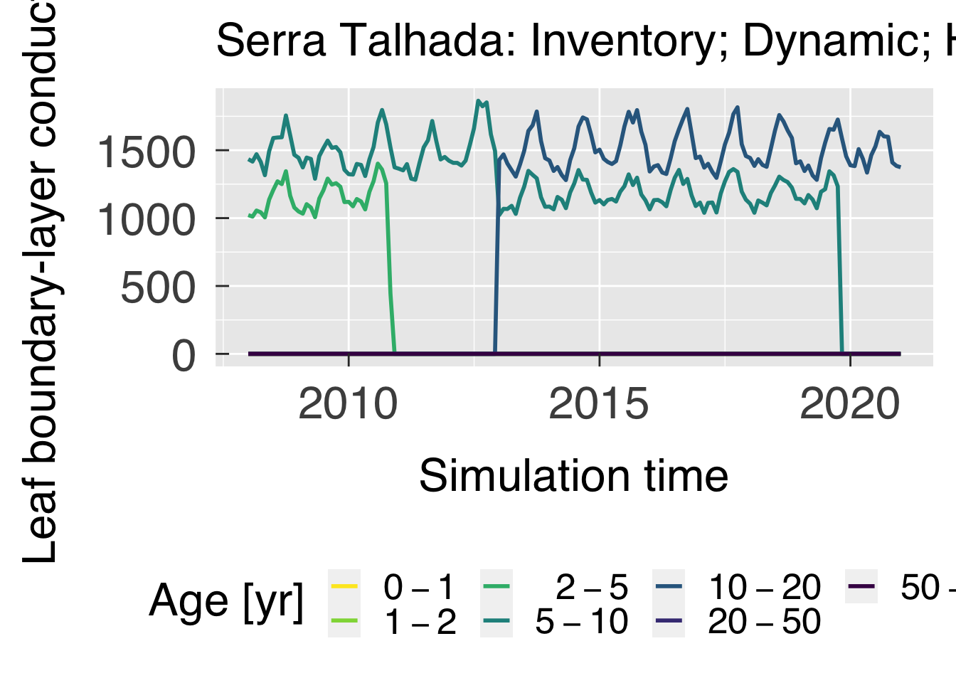
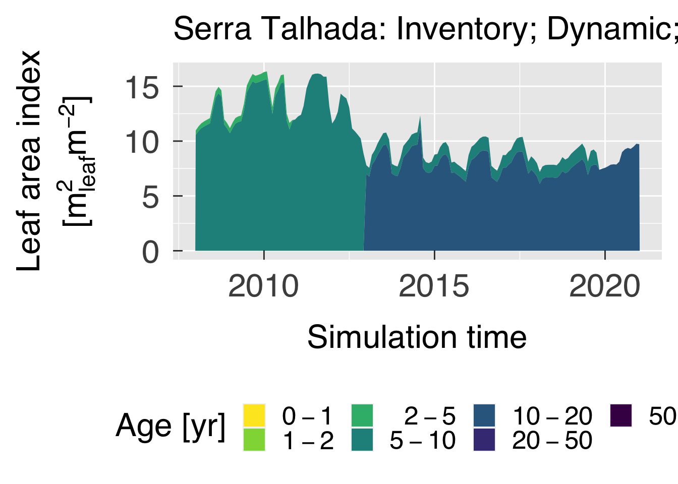
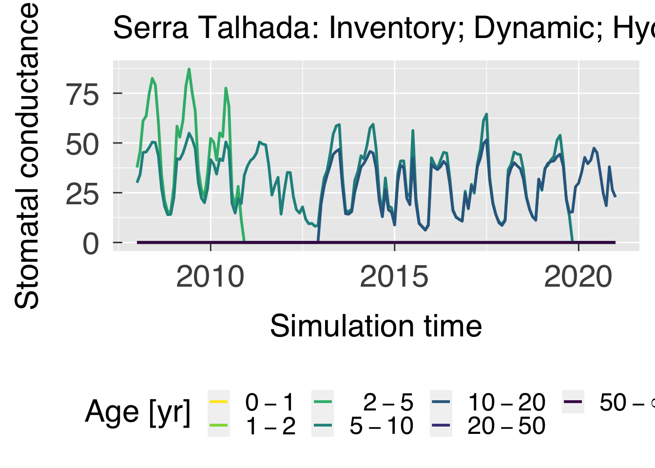
}#end if (! is_tibble(soi2d))Plot time series by age:
cat0(" + Plot time series of age-dependent variables.")

# Title for legend
age_legend = desc.unit(desc="Age",unit=untab$yr)

age_loop   = which(fatesvar$vnam %in% names(byage))
gg_age   = list()
for (f in age_loop){
  #--- Match variables.
  f_vnam   = fatesvar$vnam [f]
  f_desc   = fatesvar$desc [f]
  f_unit   = fatesvar$unit [f]
  f_stack  = fatesvar$stack[f]
  cat0("   - ",f_desc,".")
  #---~---

  #--- Temporary data table. We convert the classes back to factor.
  f_byage     = byage
  f_byage$age = factor(f_byage$age,levels=sequence(nages))
  f_colages   = ageinfo$colour
  f_agelabs   = parse(text=ageinfo$labs)
  #---~---

  #--- Initialise plot (decide whether to plot lines or stacks).
  if (f_stack){
     gg_now = ggplot(data=f_byage,aes_string(x="time",y=f_vnam,group="age",fill="age"))
     gg_now = gg_now + scale_fill_manual(name=age_legend,labels=f_agelabs,values=f_colages)
     gg_now = gg_now + geom_area(position="stack",show.legend = TRUE)
  }else{
     gg_now = ggplot(data=f_byage,aes_string(x="time",y=f_vnam,group="age",colour="age"))
     gg_now = gg_now + scale_colour_manual(name=age_legend,labels=f_agelabs,values=f_colages)
     gg_now = gg_now + geom_line(lwd=1.0,show.legend = TRUE)
  }#end if (f_stack)
  gg_now = gg_now + labs(title=case_desc)
  gg_now = gg_now + scale_x_datetime(date_labels=gg_tfmt)
  gg_now = gg_now + xlab("Simulation time")
  gg_now = gg_now + ylab(desc.unit(desc=f_desc,unit=untab[[f_unit]],twolines=TRUE))
  gg_now = gg_now + theme_grey( base_size = gg_ptsz, base_family = "Helvetica",base_line_size = 0.5,base_rect_size =0.5)
  gg_now = gg_now + theme( legend.position   = "bottom"
                         , axis.text.x       = element_text( size   = gg_ptsz
                                                           , margin = unit(rep(0.35,times=4),"cm")
                                                           )#end element_text
                         , axis.text.y       = element_text( size   = gg_ptsz
                                                           , margin = unit(rep(0.35,times=4),"cm")
                                                           )#end element_text
                         , plot.title        = element_text( size = gg_ptsz)
                         , axis.ticks.length = unit(-0.25,"cm")
                         )#end theme
  #---~---

  #--- Save plot.
  for (d in sequence(ndevice)){
    f_output = paste0(f_vnam,"-tsage-",case_fpref,".",gg_device[d])
    dummy = ggsave( filename = f_output
                  , plot     = gg_now
                  , device   = gg_device[d]
                  , path     = tsage_path
                  , width    = gg_width
                  , height   = gg_height
                  , units    = gg_units
                  , dpi      = gg_depth
                  )#end ggsave
  }#end for (o in sequence(nout))
  #---~---

  #--- Write plot settings to the list.
  gg_age[[f_vnam]] = gg_now
  #---~---
}#end for (a in age_loop)
## Warning: `aes_string()` was deprecated in ggplot2 3.0.0.
## ℹ Please use tidy evaluation idioms with `aes()`.
## ℹ See also `vignette("ggplot2-in-packages")` for more information.
## This warning is displayed once every 8 hours.
## Call `lifecycle::last_lifecycle_warnings()` to see where this warning was
## generated.#--- If sought, plot images on screen
if (gg_screen) gg_age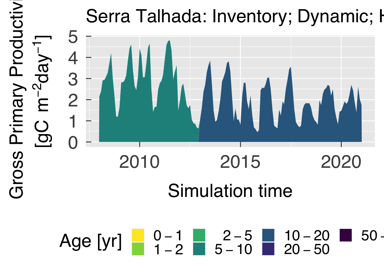
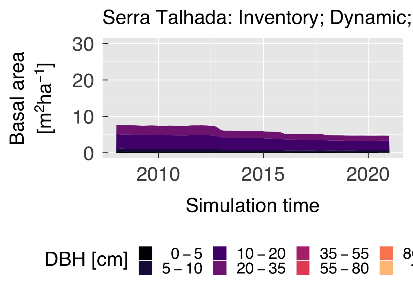
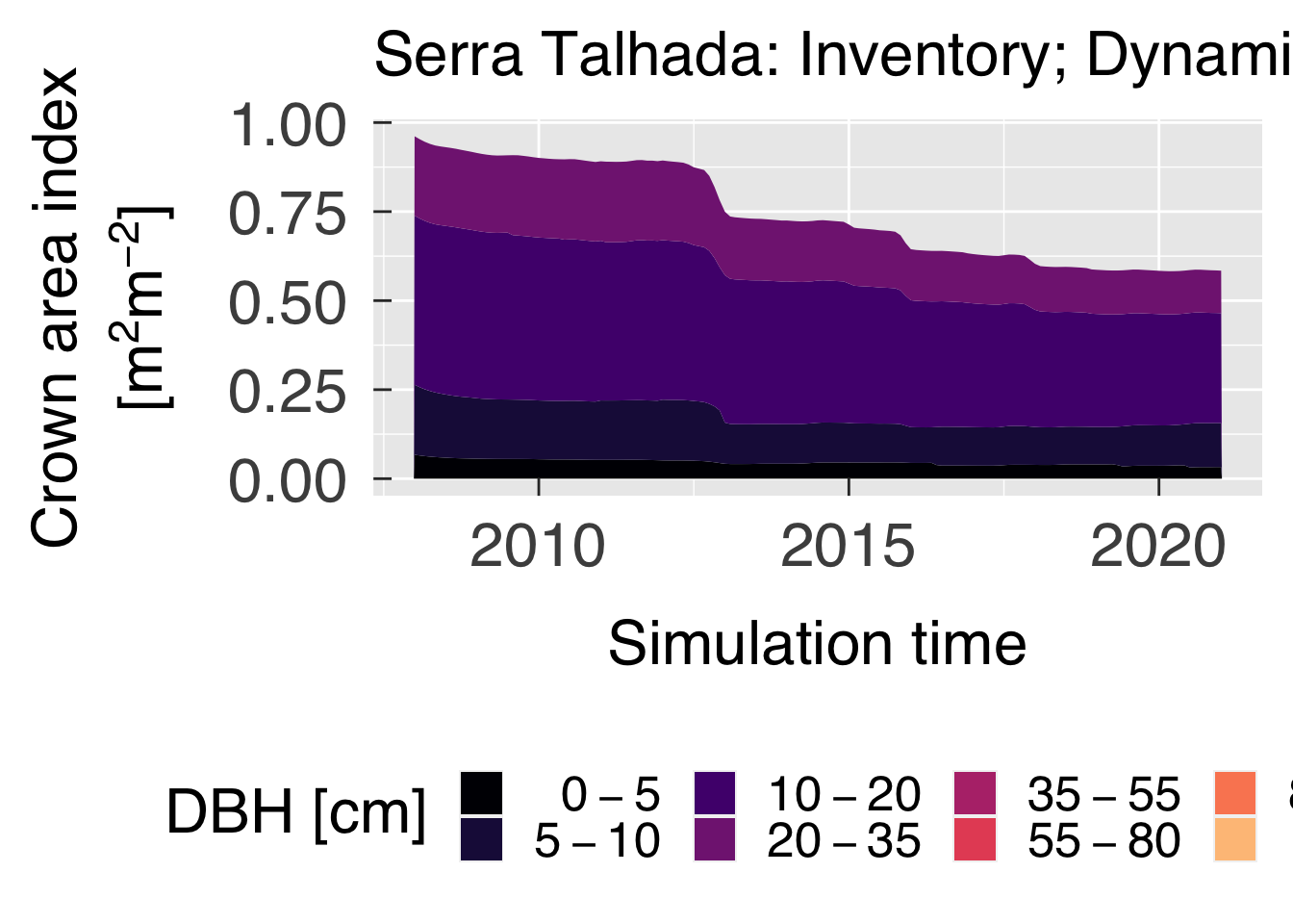
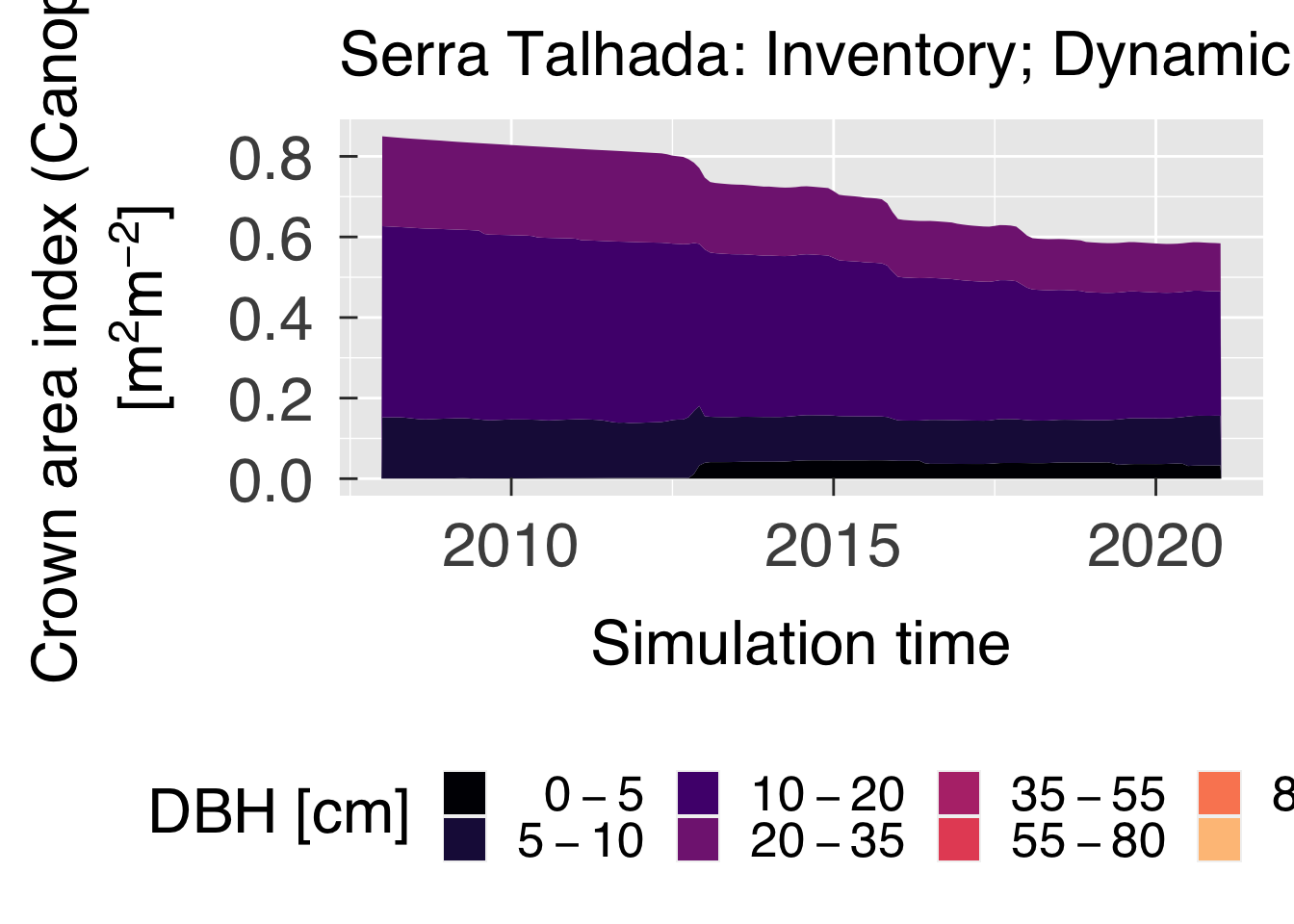
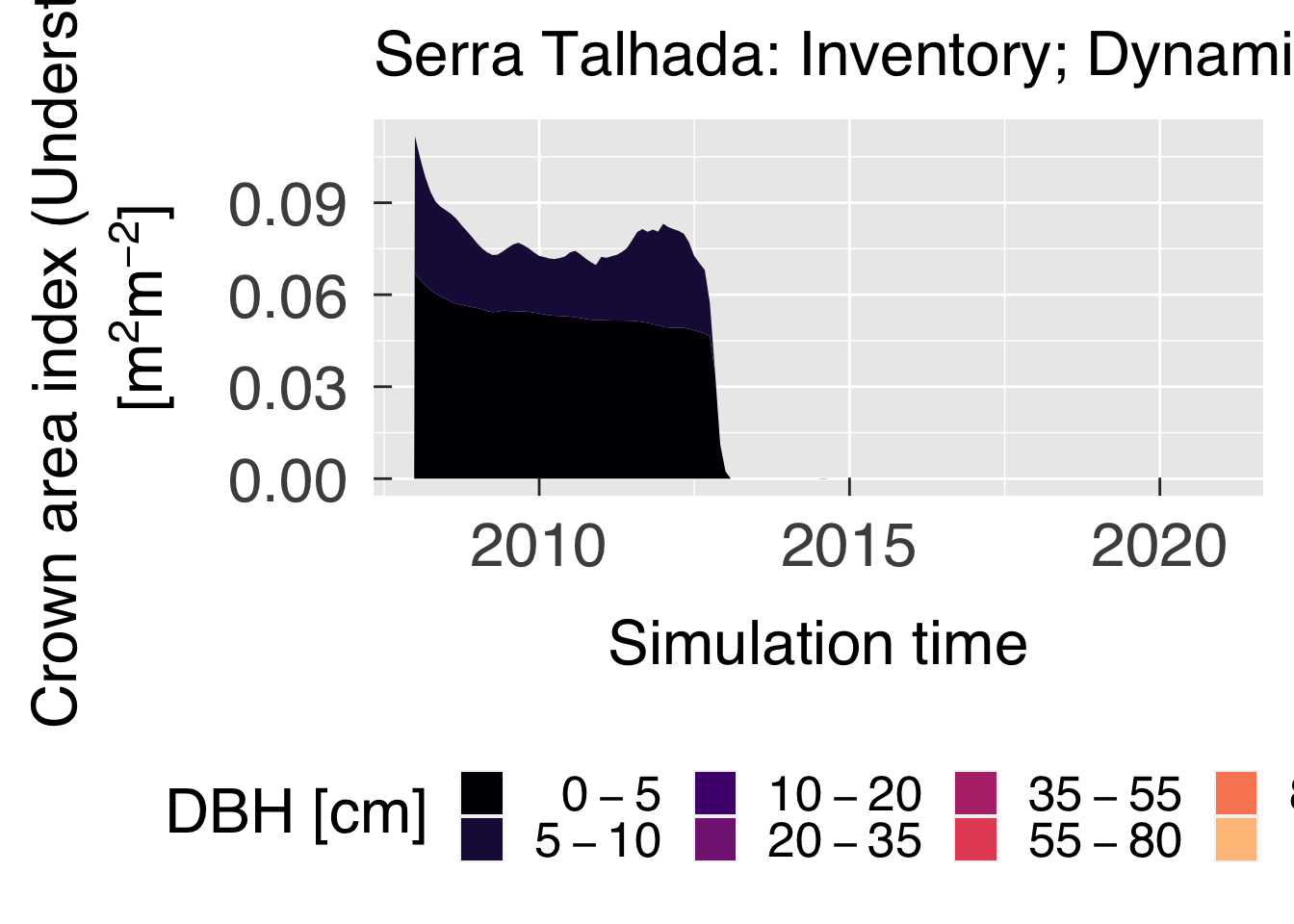
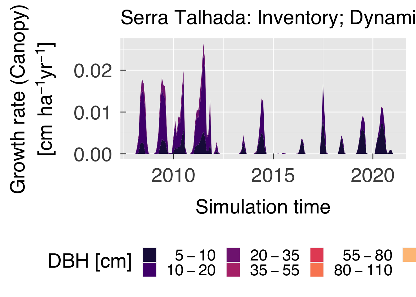
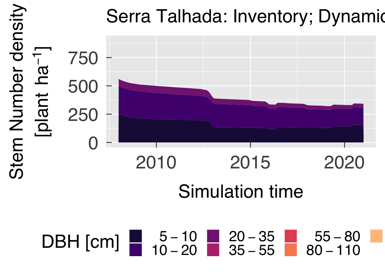
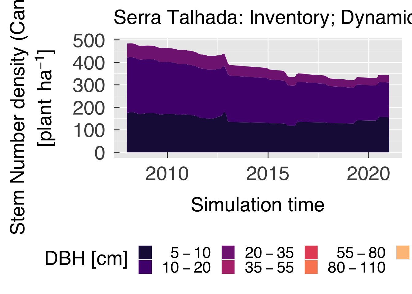
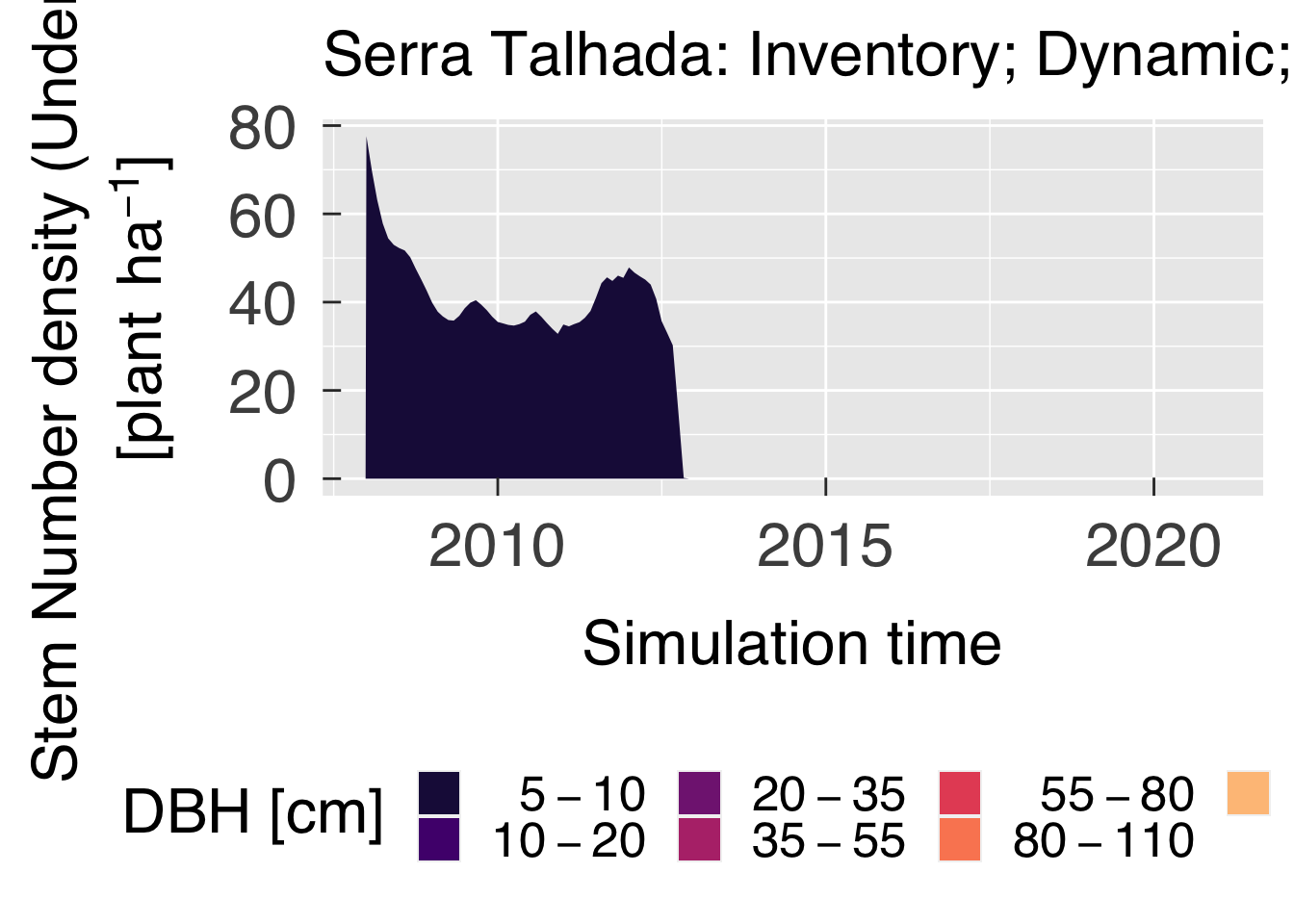
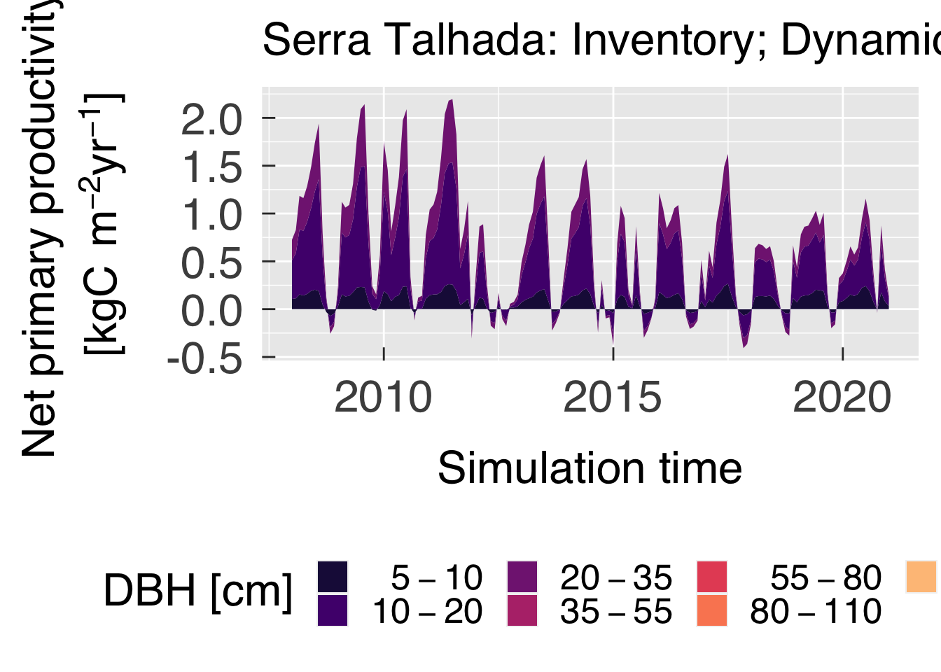
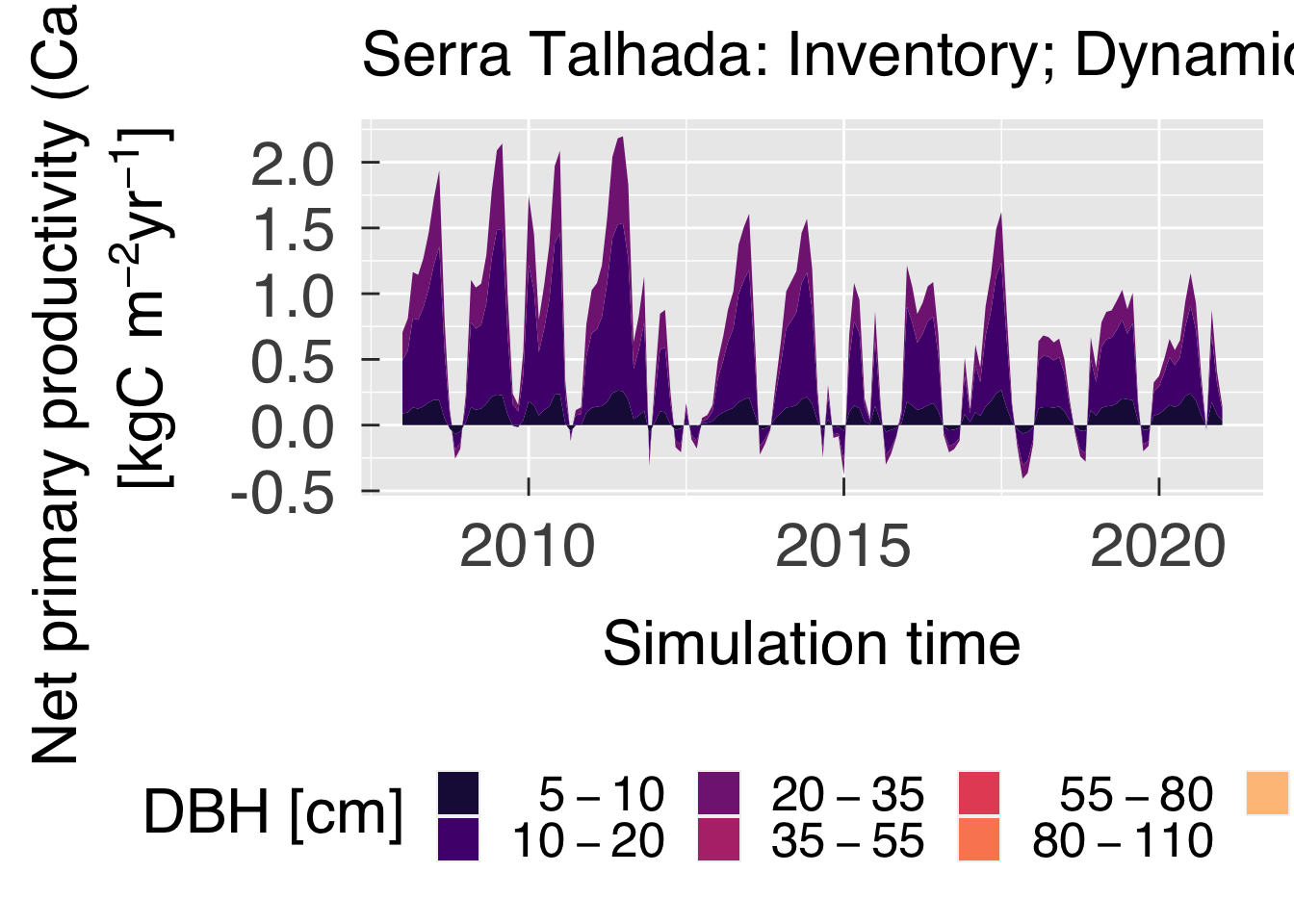
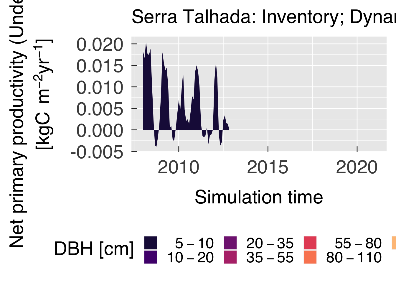
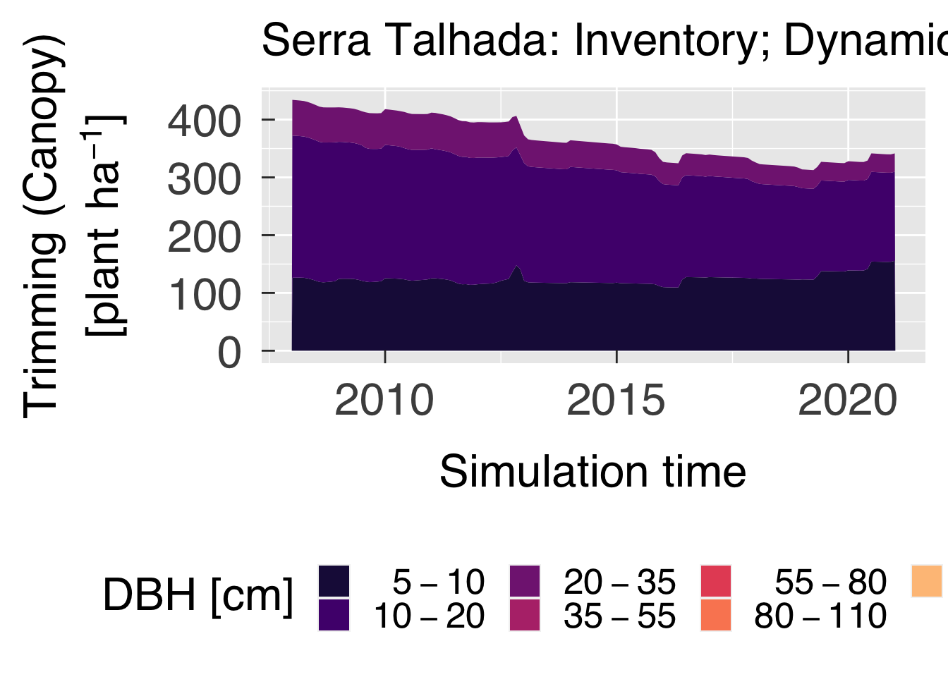
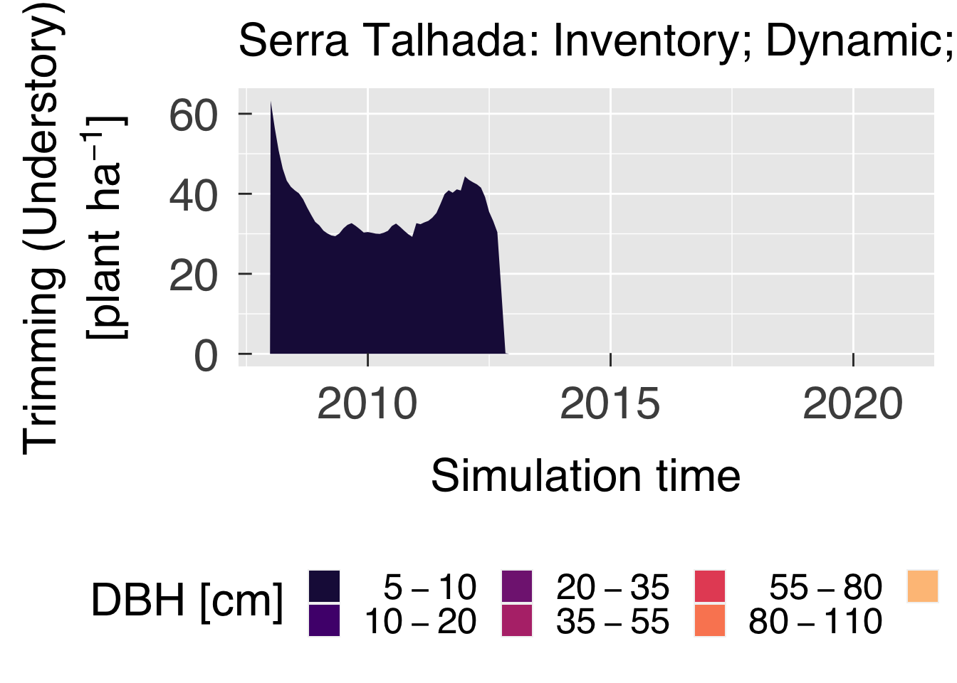
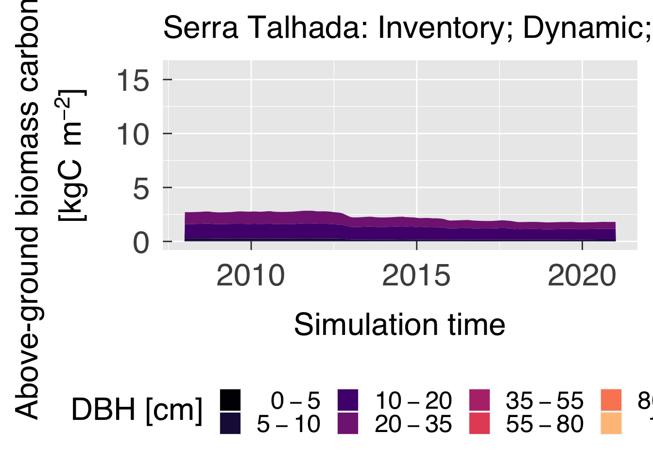
#---~---Plot time series by size class:
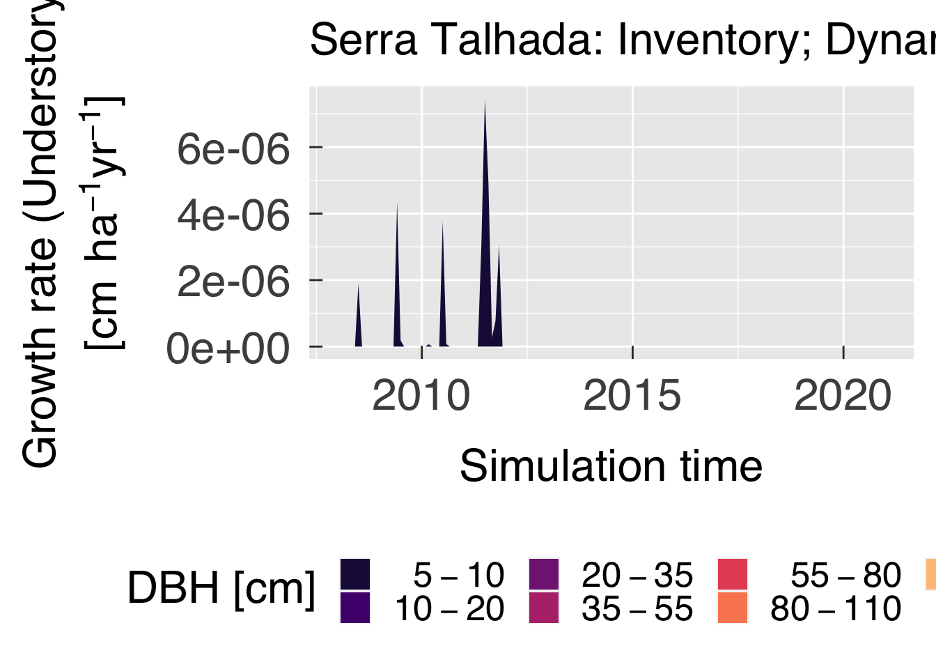
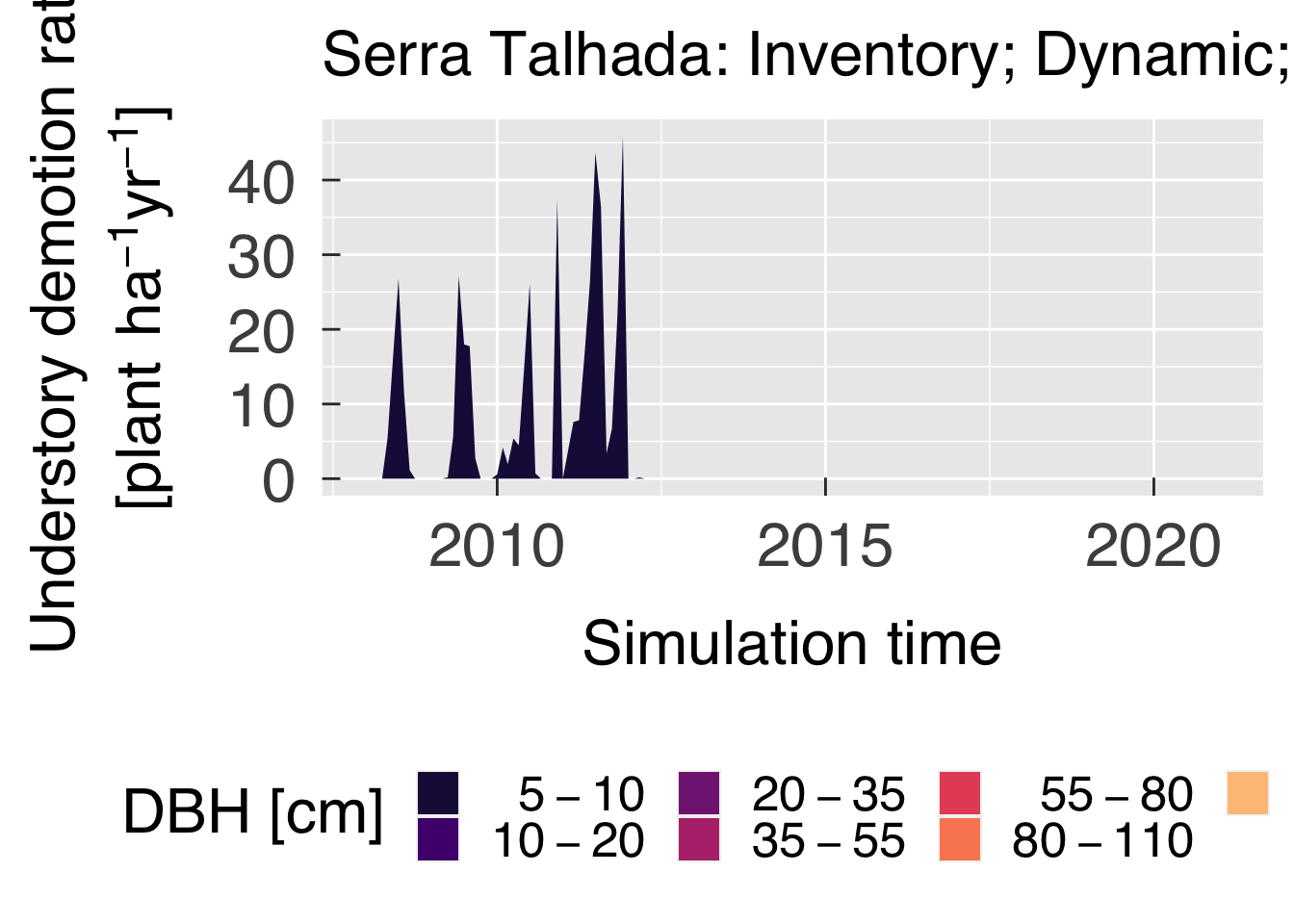
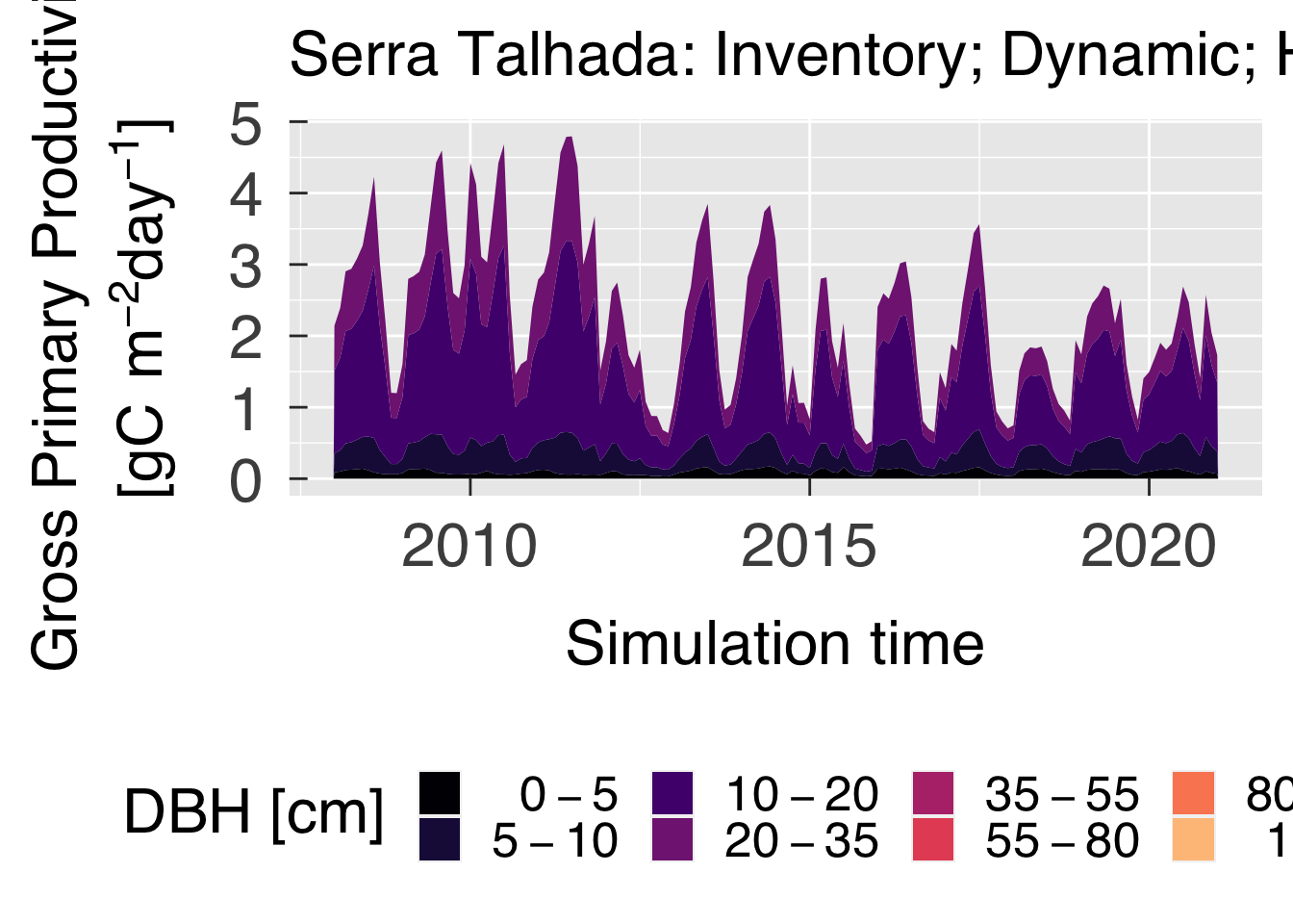
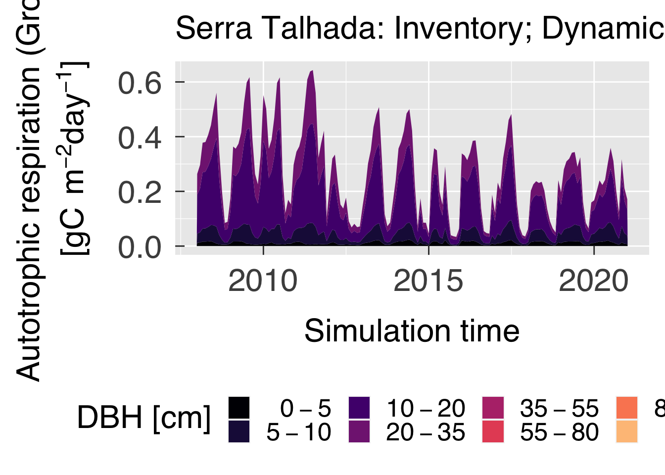
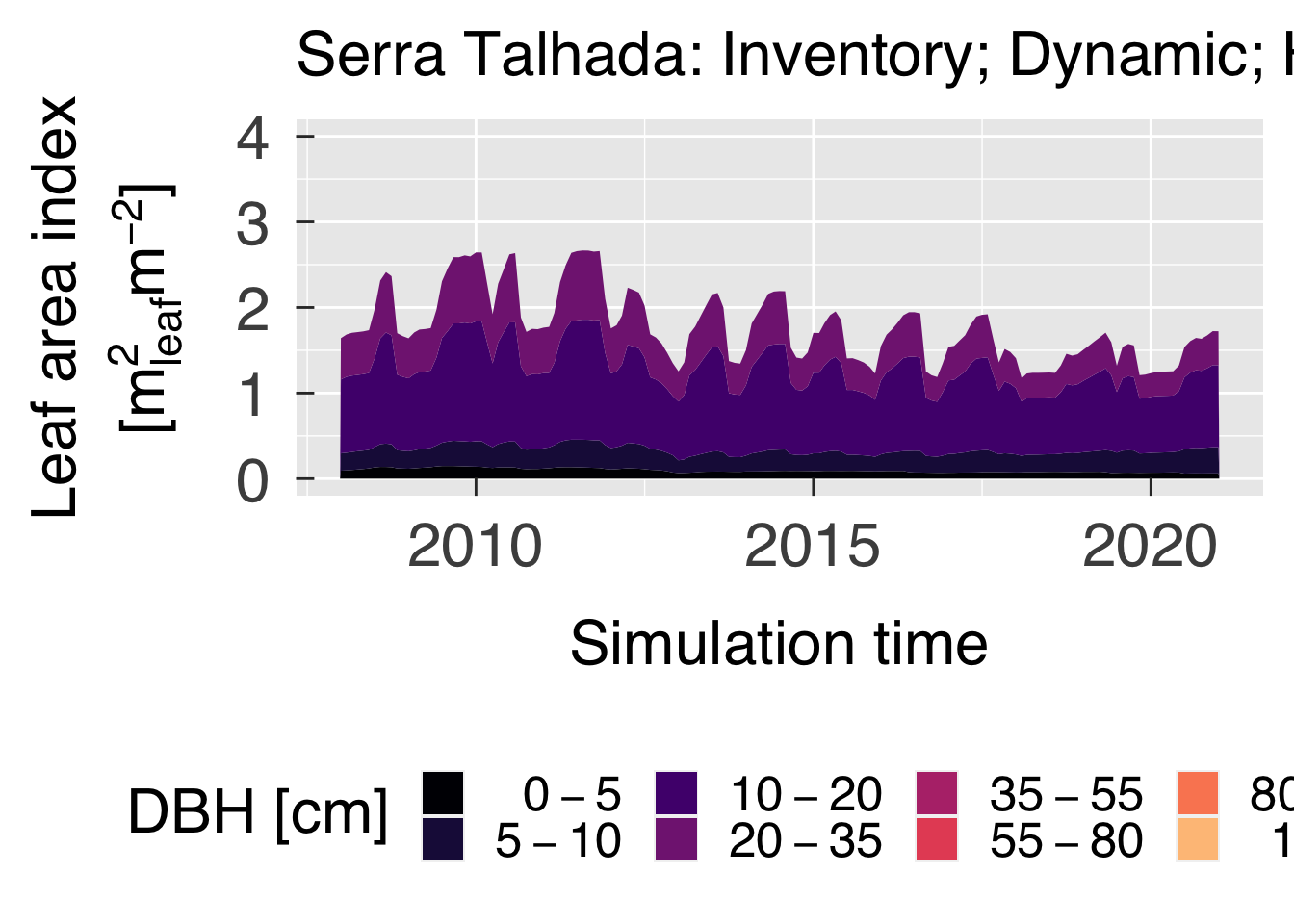
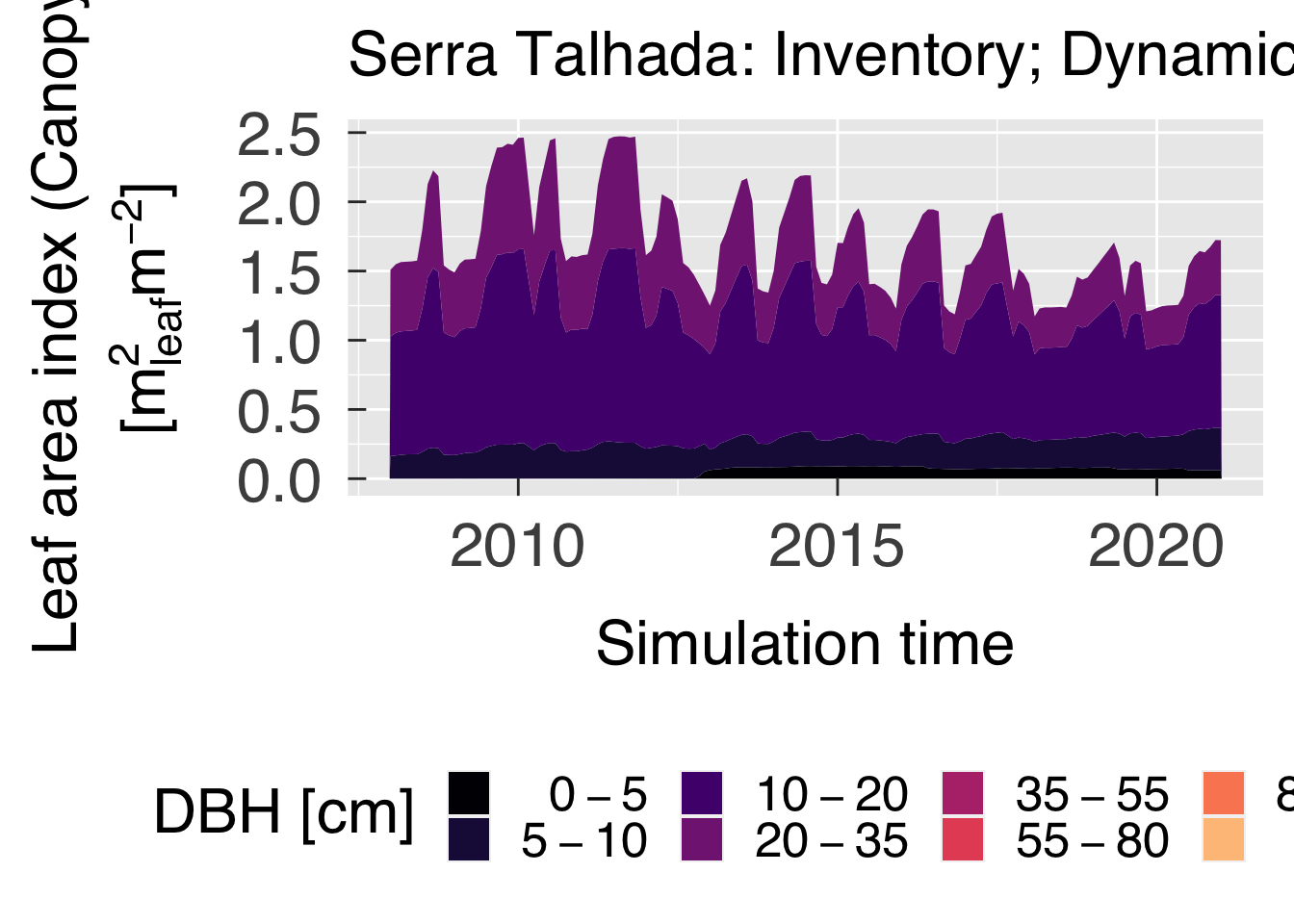
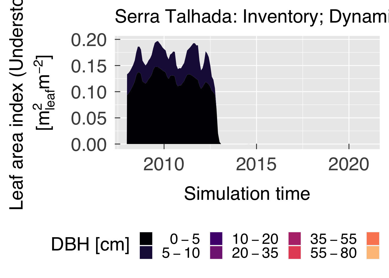
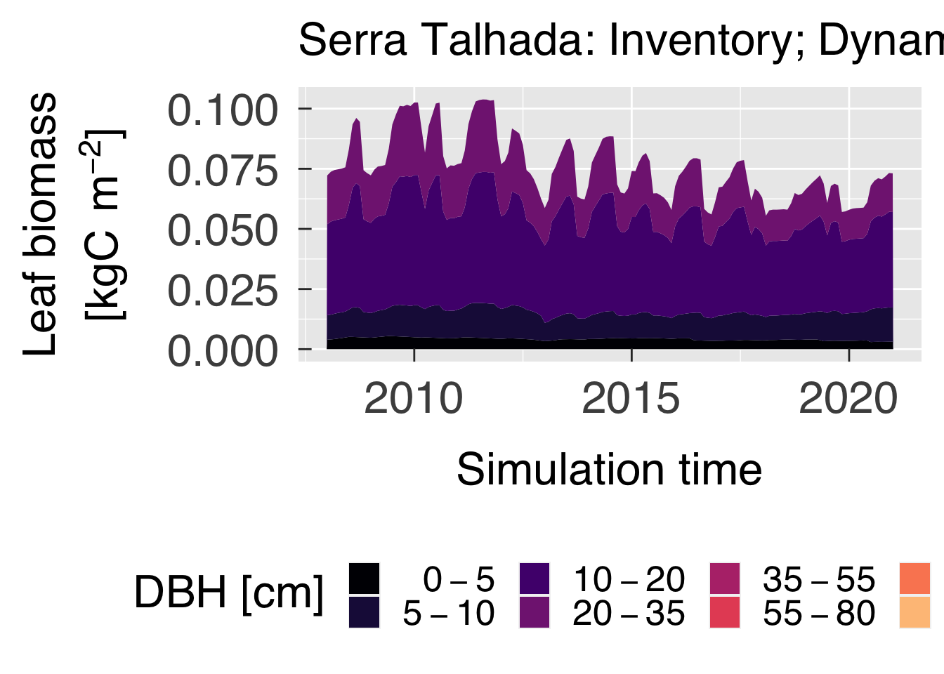
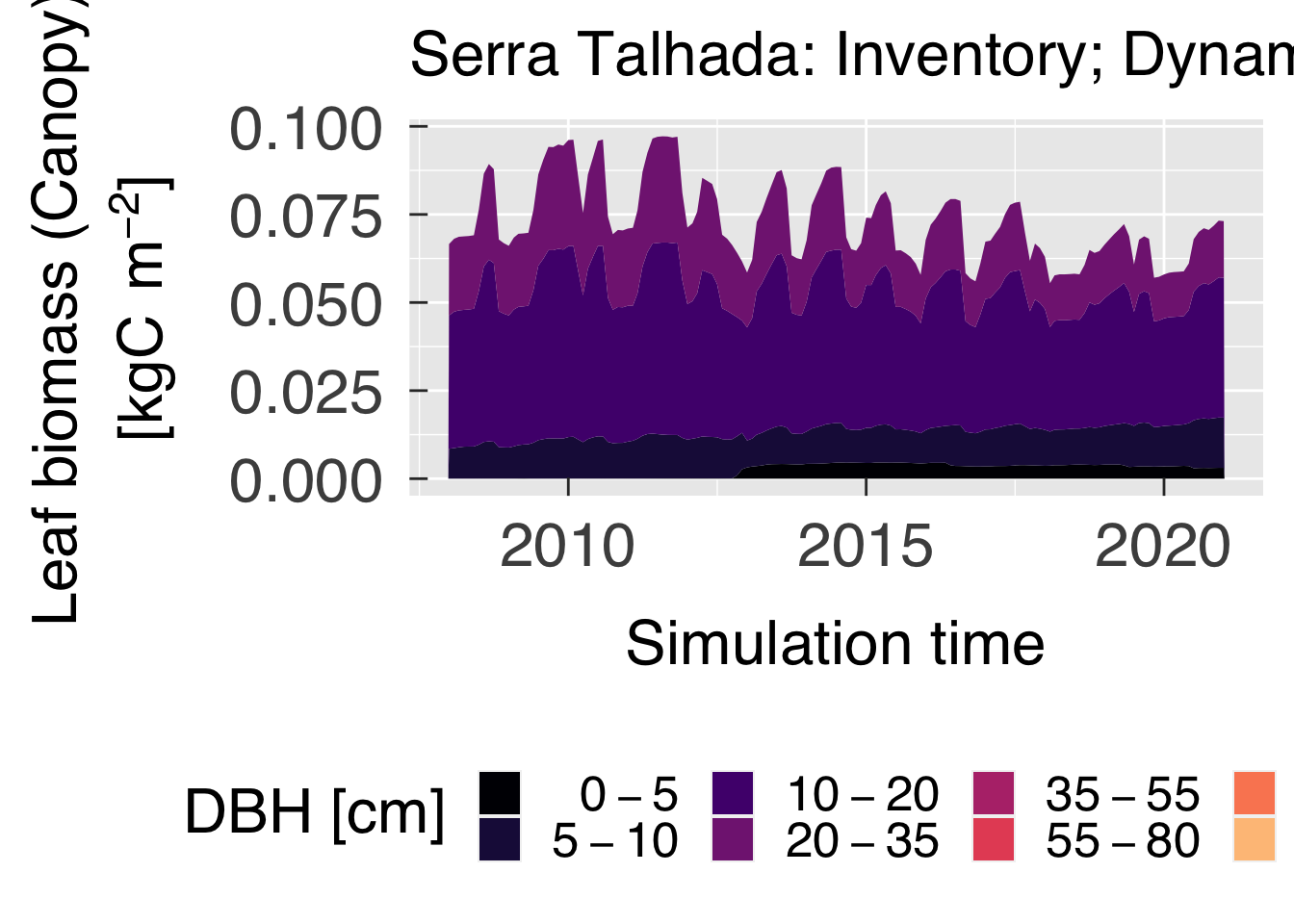
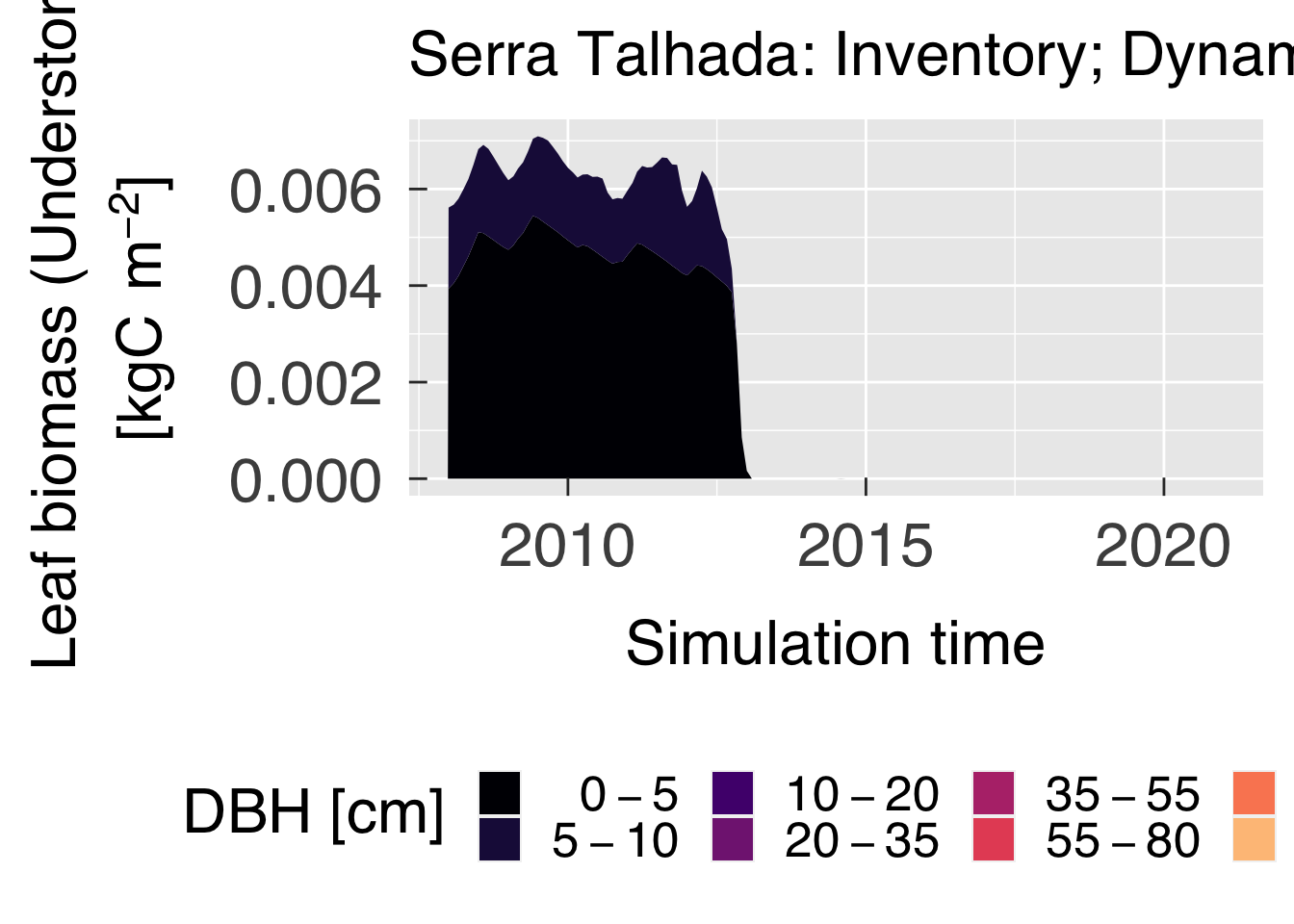
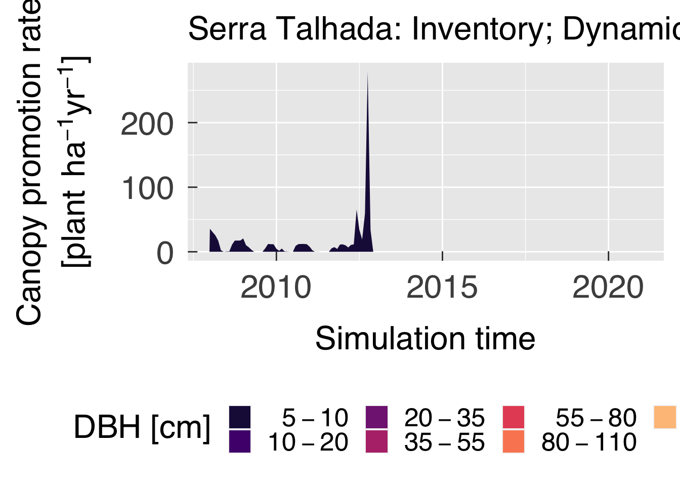
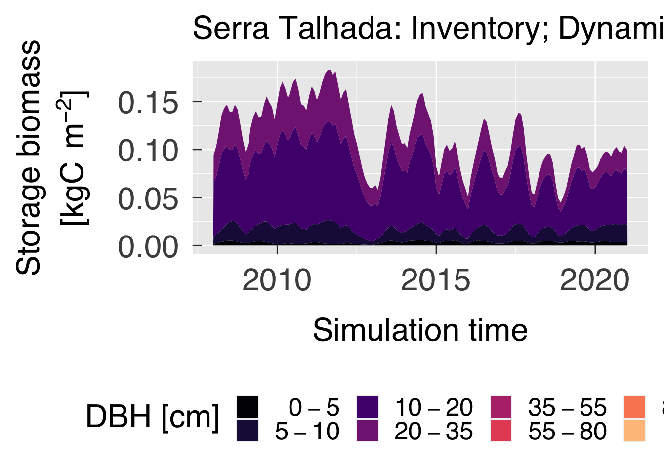
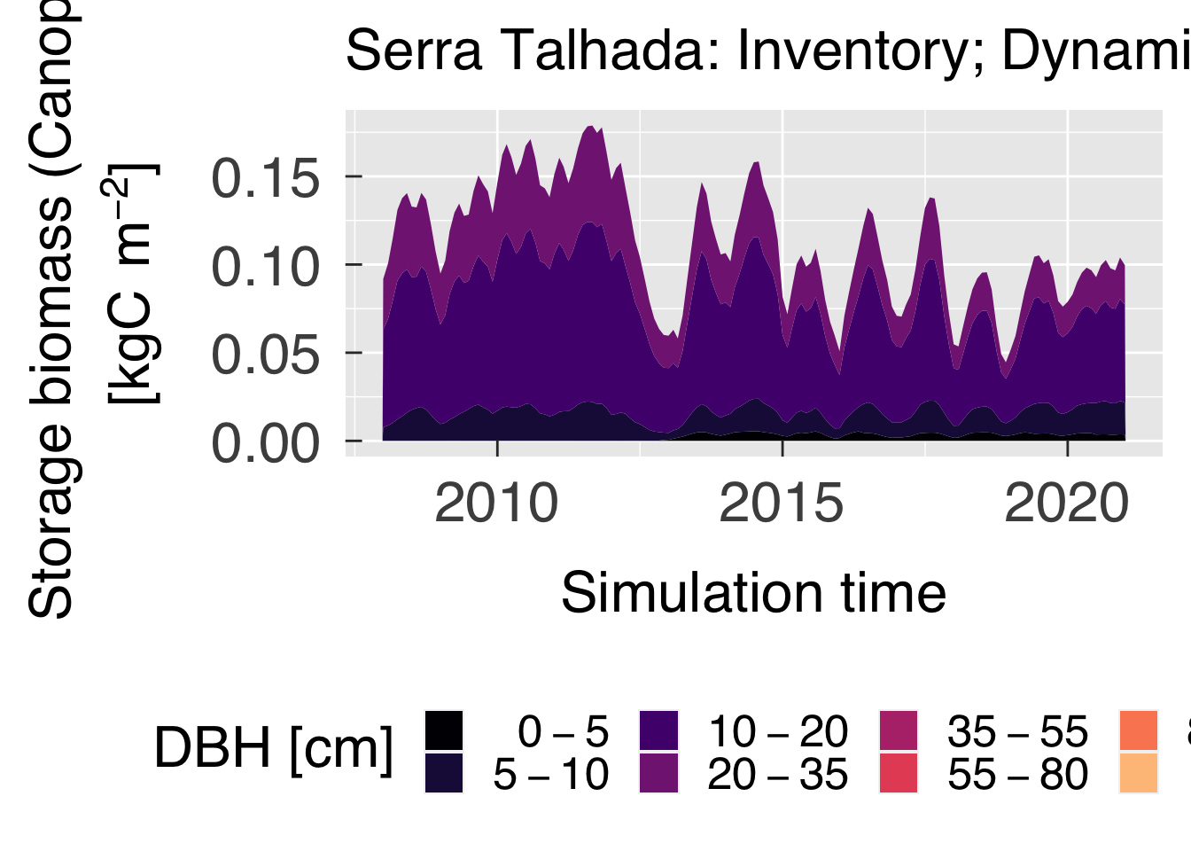
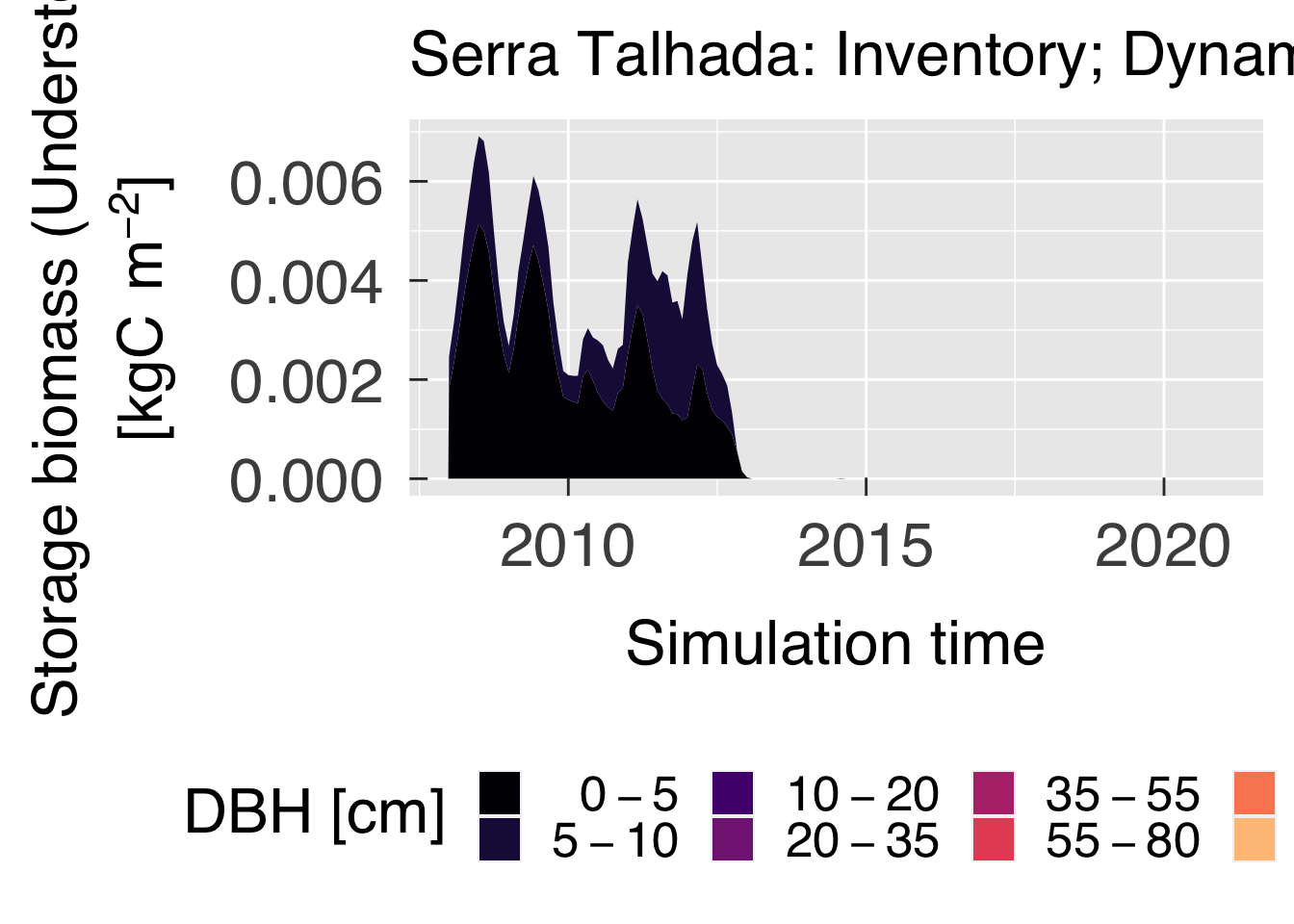
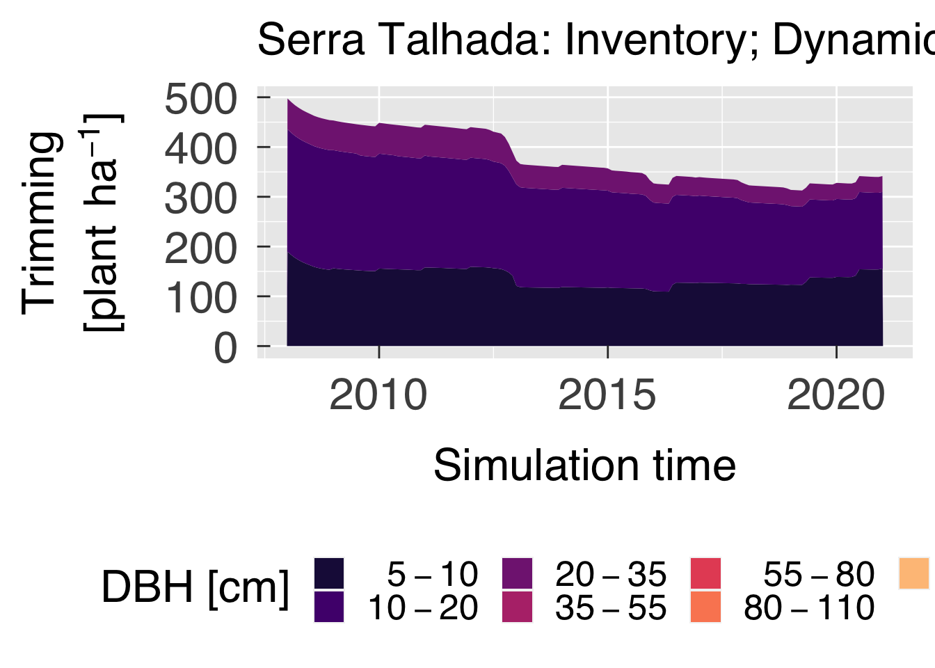
cat0(" + Plot time series of size-dependent variables.")

#--- Title for legend
dbh_legend = desc.unit(desc="DBH",unit=untab$cm)
#---~---

dbh_loop = which(fatesvar$vnam %in% names(bydbh))
gg_dbh   = list()
for (f in dbh_loop){
  #--- Match variables.
  f_vnam   = fatesvar$vnam  [f]
  f_desc   = fatesvar$desc  [f]
  f_unit   = fatesvar$unit  [f]
  f_stack  = fatesvar$stack [f]
  f_dbh01  = fatesvar$dbh01 [f]
  f_ylower = fatesvar$ylower[f]
  f_yupper = fatesvar$yupper[f]
  cat0("   - ",f_desc,".")
  #---~---

  #--- Decide whether to plot the first class.
  if (f_dbh01){
    #--- Keep all classes.
    f_bydbh     = bydbh
    f_bydbh$dbh = factor(f_bydbh$dbh,levels=sequence(ndbhs))
    f_coldbhs   = dbhinfo$colour
    f_dbhlabs   = parse(text=dbhinfo$labs)
    #---~---
  }else{
    #--- Exclude first class.
    bye         = as.numeric(bydbh$dbh) %in% 1
    f_bydbh     = bydbh[! bye,]
    f_bydbh$dbh = factor(f_bydbh$dbh,levels=sequence(ndbhs)[-1])
    f_coldbhs   = dbhinfo$colour[-1]
    f_dbhlabs   = parse(text=dbhinfo$labs[-1])
    #---~---
  }#end if (f_dbh01)
  #---~---

  #--- Initialise plot (decide whether to plot lines or stacks).
  if (f_stack){
     gg_now = ggplot(data=f_bydbh,aes_string(x="time",y=f_vnam,group="dbh",fill="dbh"))
     gg_now = gg_now + scale_fill_manual(name=dbh_legend,labels=f_dbhlabs,values=f_coldbhs)
     gg_now = gg_now + geom_area(position=position_stack(reverse = TRUE),show.legend = TRUE)
  }else{
     gg_now = ggplot(data=f_bydbh,aes_string(x="time",y=f_vnam,group="dbh",colour="dbh"))
     gg_now = gg_now + scale_colour_manual(name=dbh_legend,labels=f_dbhlabs,values=f_coldbhs)
     gg_now = gg_now + geom_line(lwd=1.0,show.legend = TRUE)
  }#end if (f_stack)
  gg_now = gg_now + labs(title=case_desc)
  gg_now = gg_now + scale_x_datetime(date_labels=gg_tfmt)
  if (all(is.finite(c(f_ylower,f_yupper)))){
     gg_now = gg_now + scale_y_continuous(limits=c(f_ylower,f_yupper),oob=oob_keep)
  }#end if (all(is.finite(f_ylower,f_yupper)))
  gg_now = gg_now + xlab("Simulation time")
  gg_now = gg_now + ylab(desc.unit(desc=f_desc,unit=untab[[f_unit]],twolines=TRUE))
  gg_now = gg_now + theme_grey( base_size = gg_ptsz, base_family = "Helvetica",base_line_size = 0.5,base_rect_size =0.5)
  gg_now = gg_now + theme( legend.position   = "bottom"
                         , axis.text.x       = element_text( size   = gg_ptsz
                                                           , margin = unit(rep(0.35,times=4),"cm")
                                                           )#end element_text
                         , axis.text.y       = element_text( size   = gg_ptsz
                                                           , margin = unit(rep(0.35,times=4),"cm")
                                                           )#end element_text
                         , plot.title        = element_text( size = gg_ptsz)
                         , axis.ticks.length = unit(-0.25,"cm")
                         )#end theme
  #---~---

  #--- Save plot.
  for (d in sequence(ndevice)){
    f_output = paste0(f_vnam,"-tsdbh-",case_fpref,".",gg_device[d])
    dummy = ggsave( filename = f_output
                  , plot     = gg_now
                  , device   = gg_device[d]
                  , path     = tsdbh_path
                  , width    = gg_width
                  , height   = gg_height
                  , units    = gg_units
                  , dpi      = gg_depth
                  )#end ggsave
  }#end for (o in sequence(nout))
  #---~---

  #--- Write plot settings to the list.
  gg_dbh[[f_vnam]] = gg_now
  #---~---
}#end for (a in age_loop)


#--- If sought, plot images on screen
if (gg_screen) gg_dbh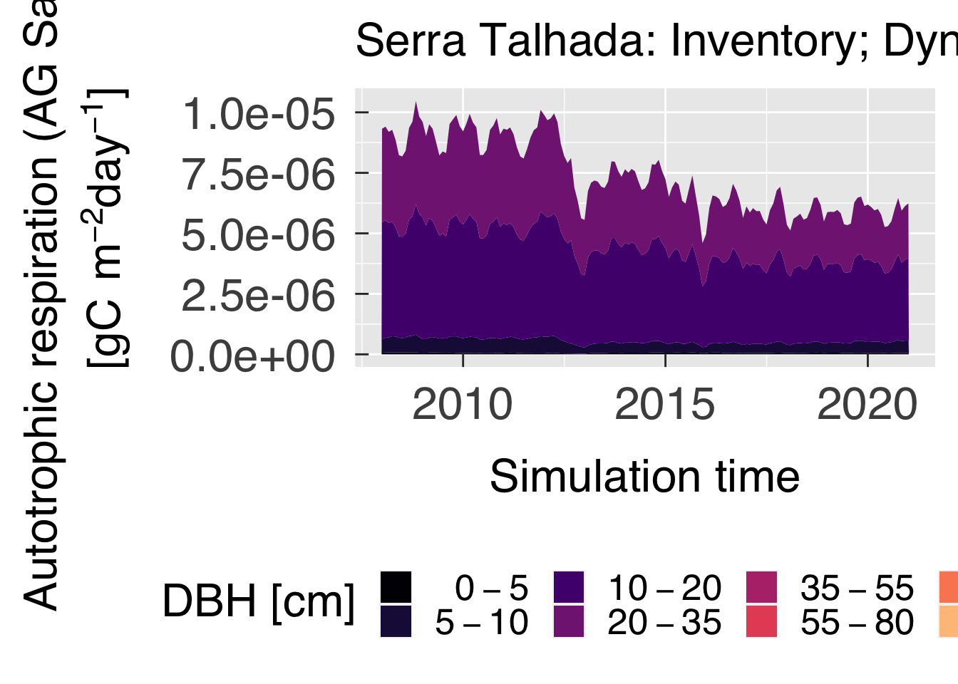
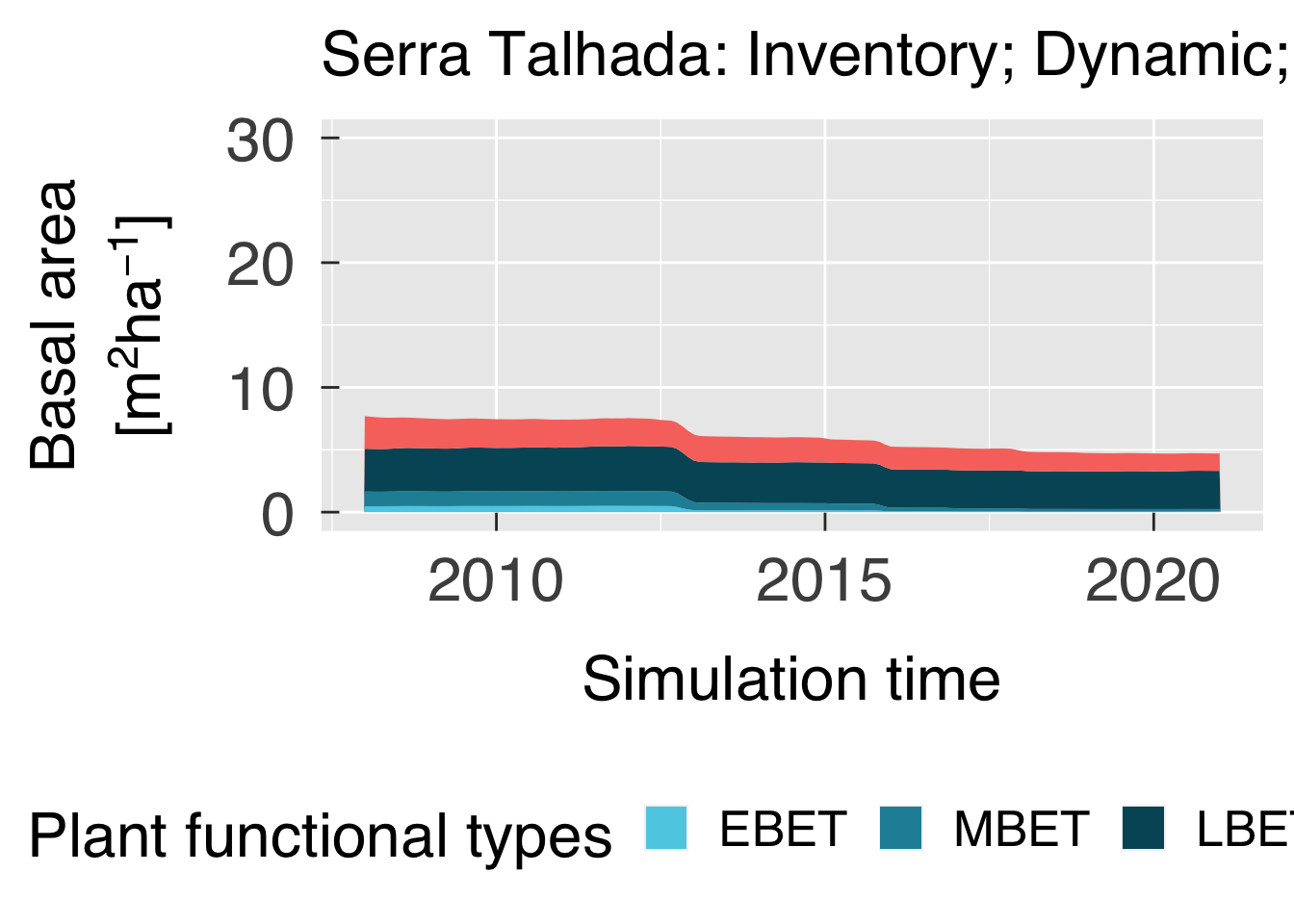
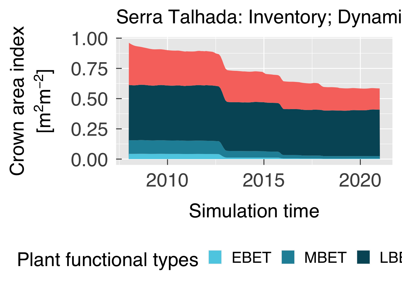
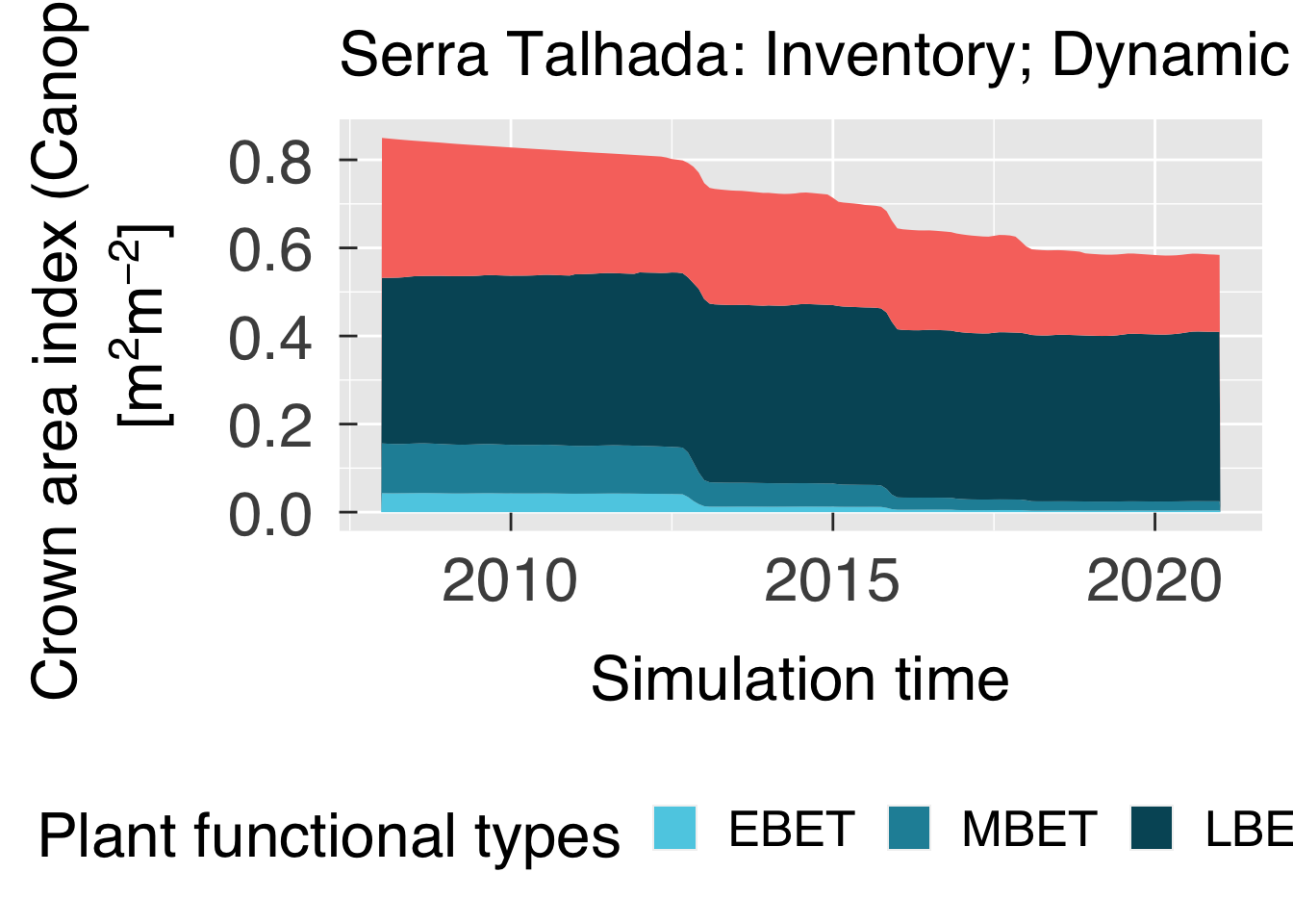
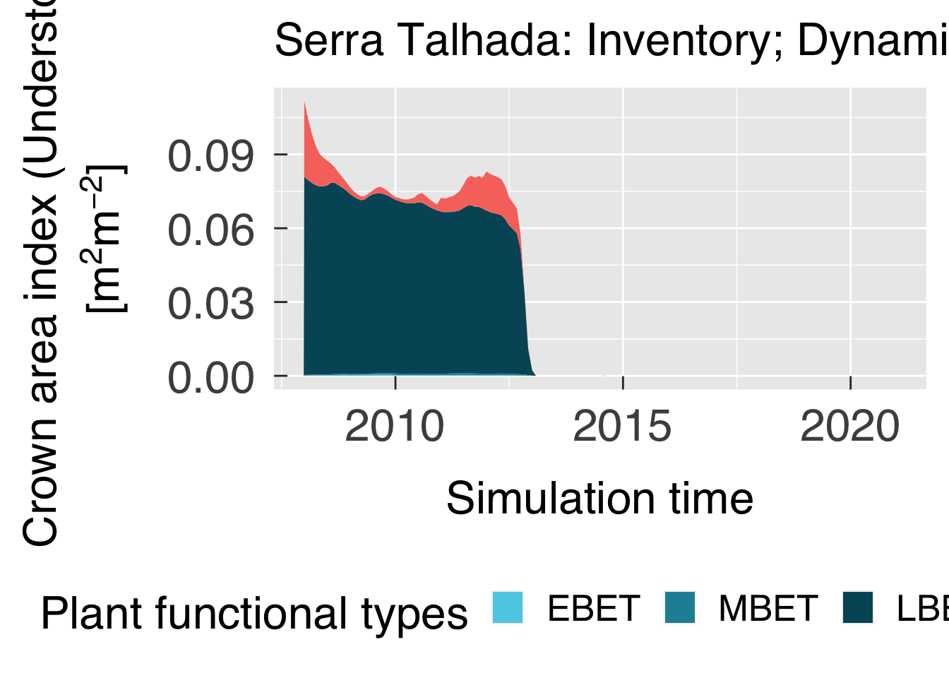
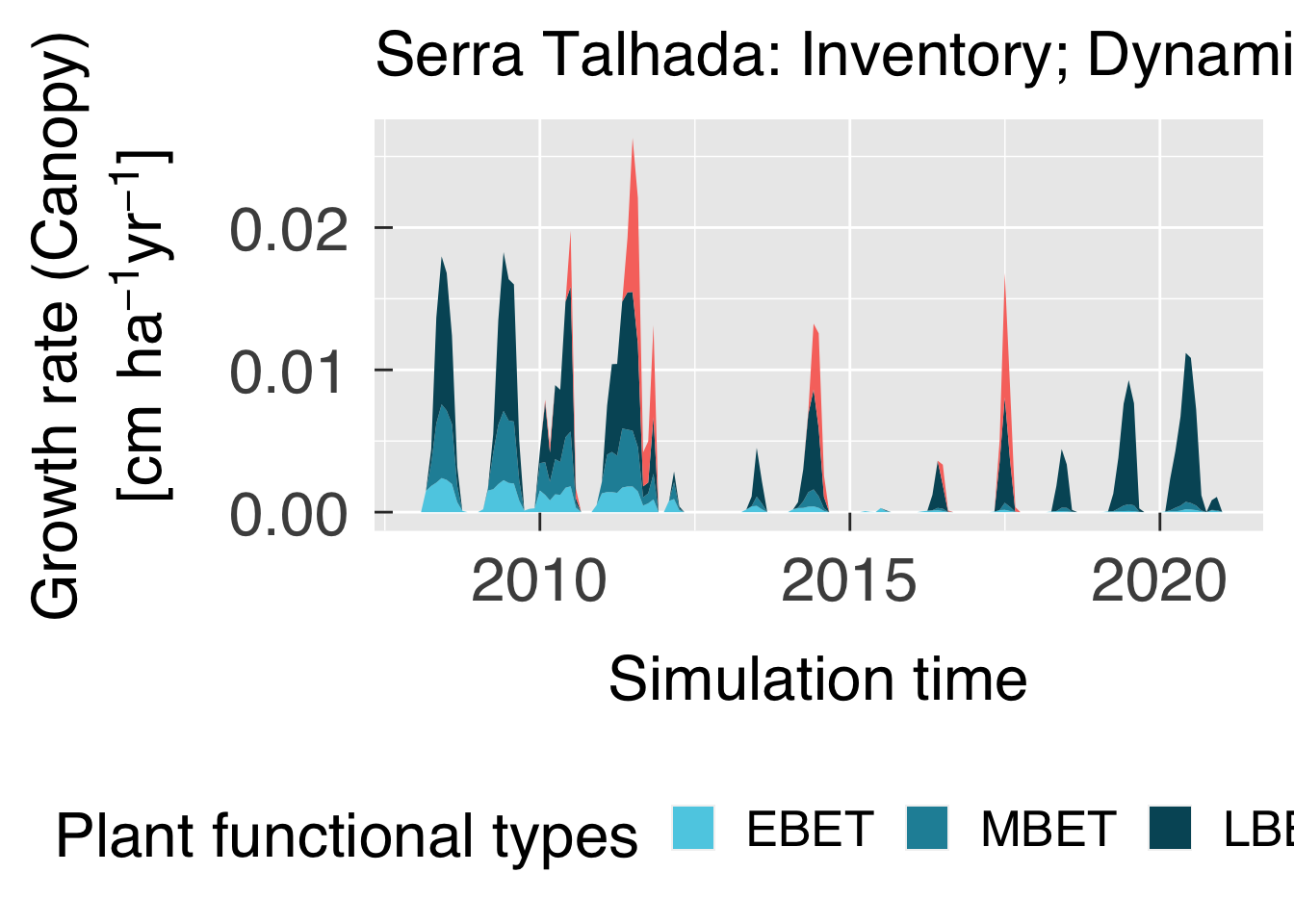
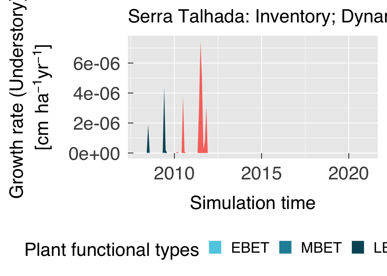
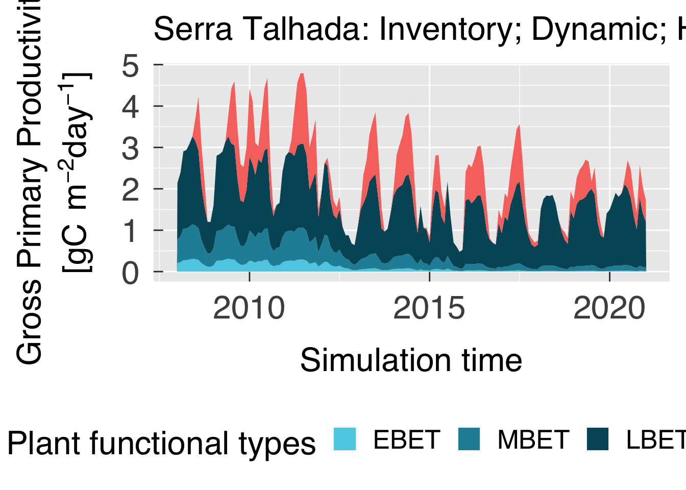
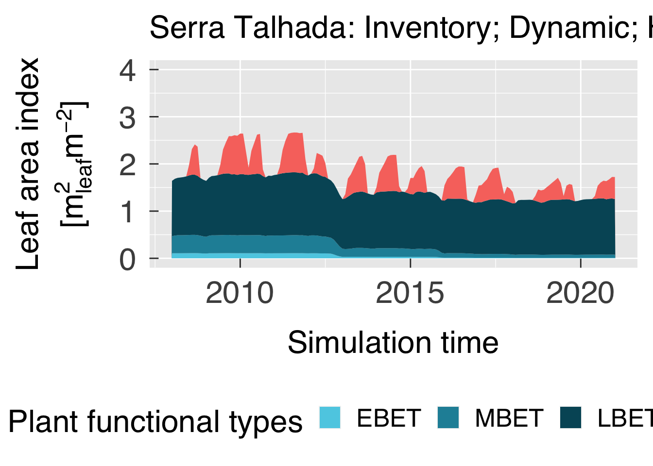
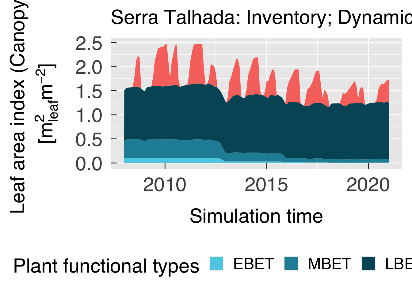
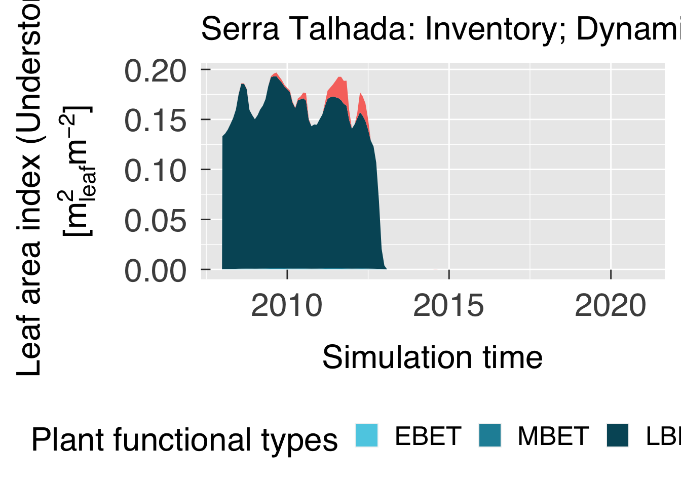
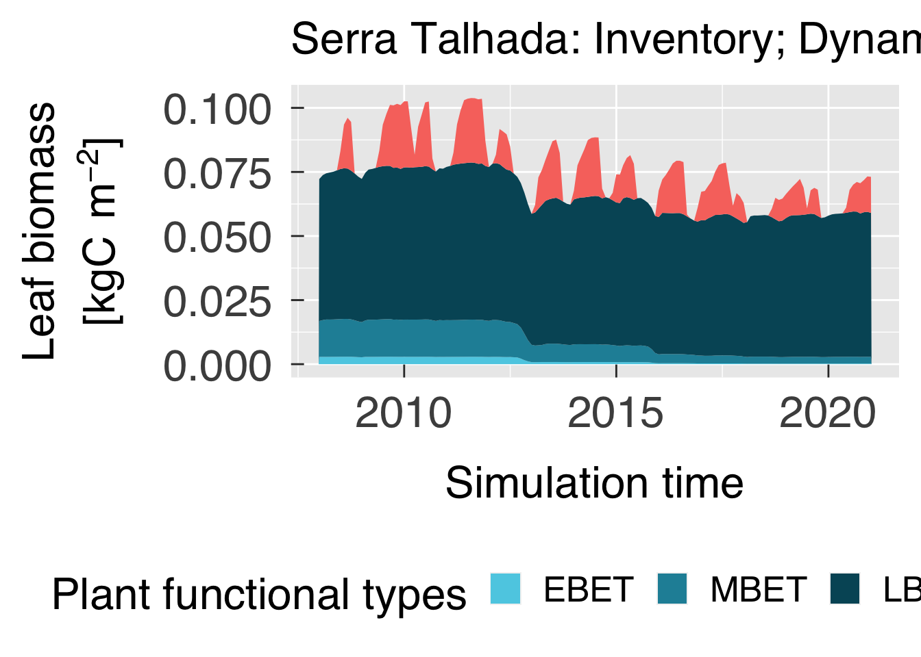
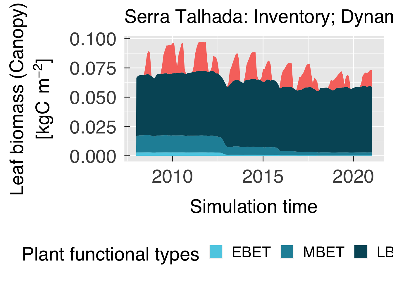
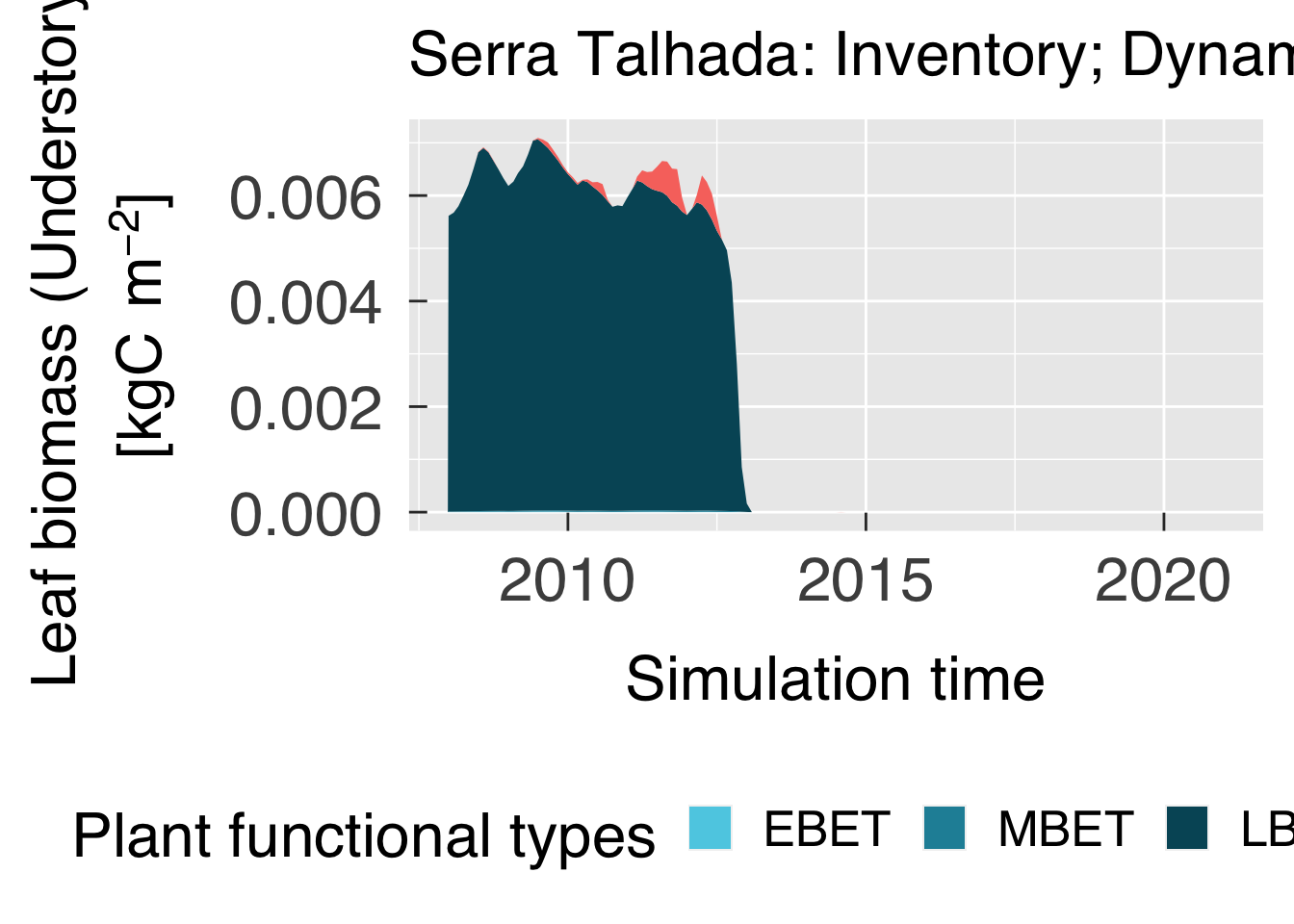
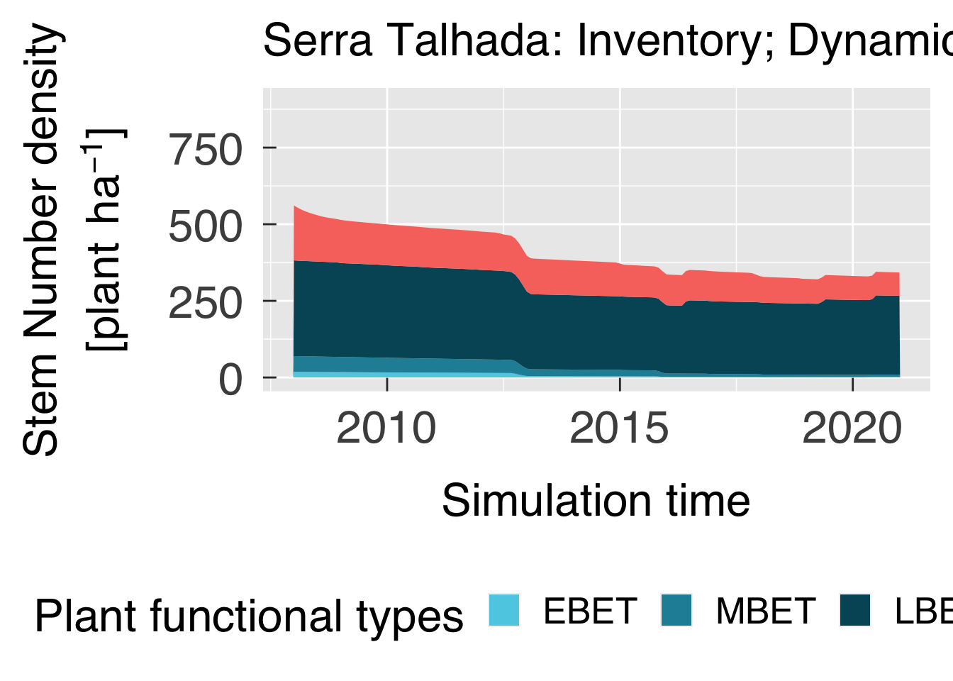
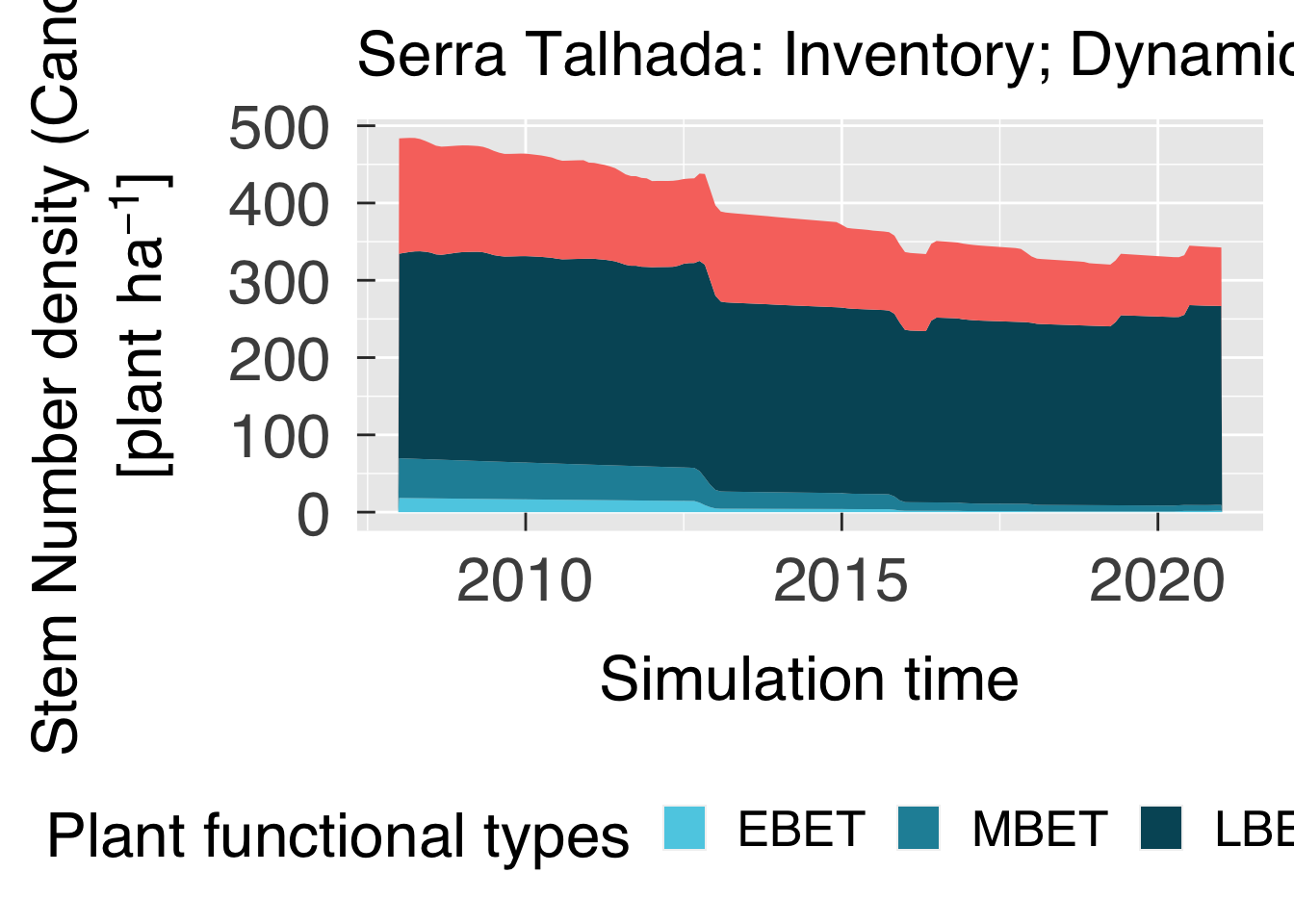
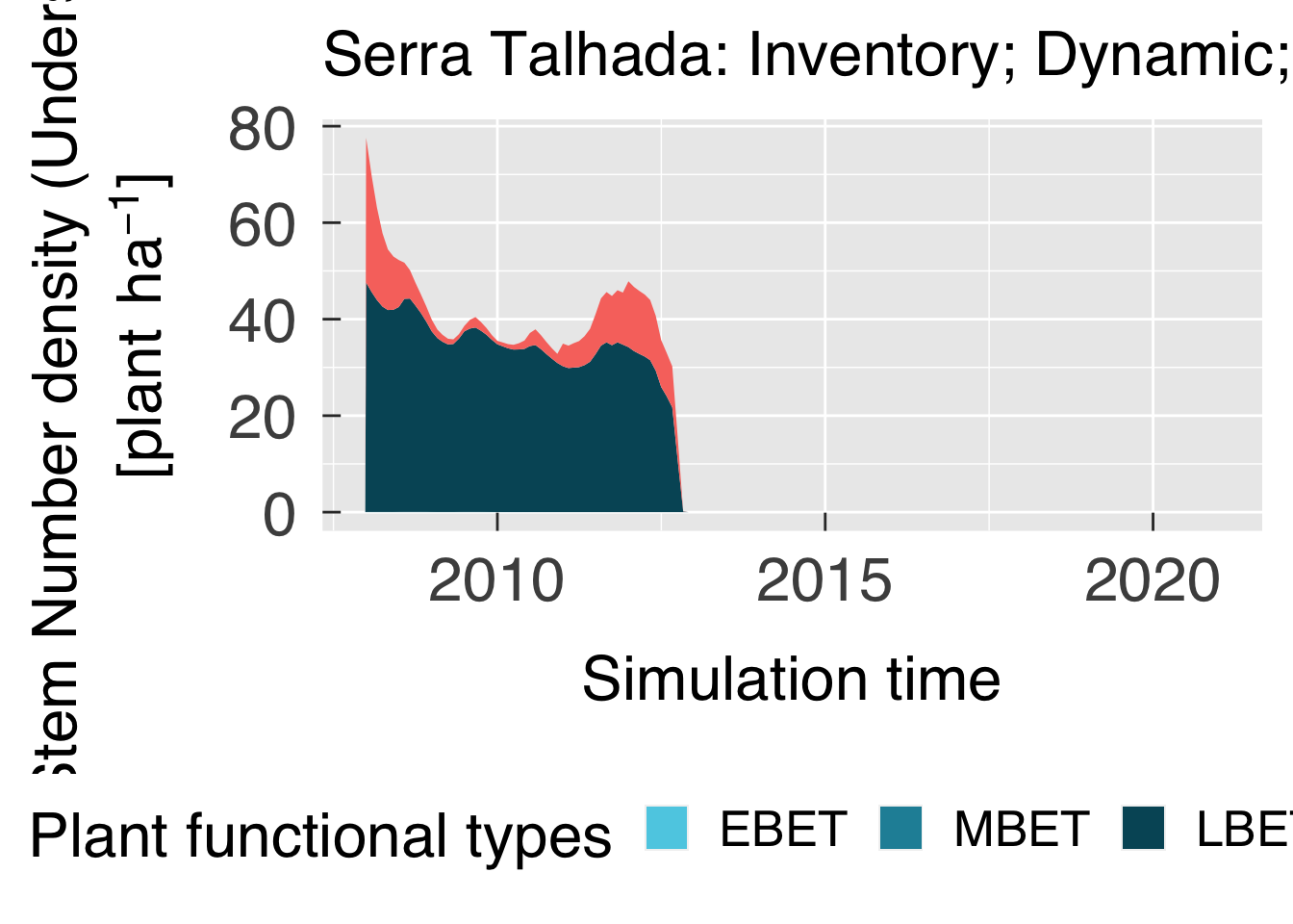
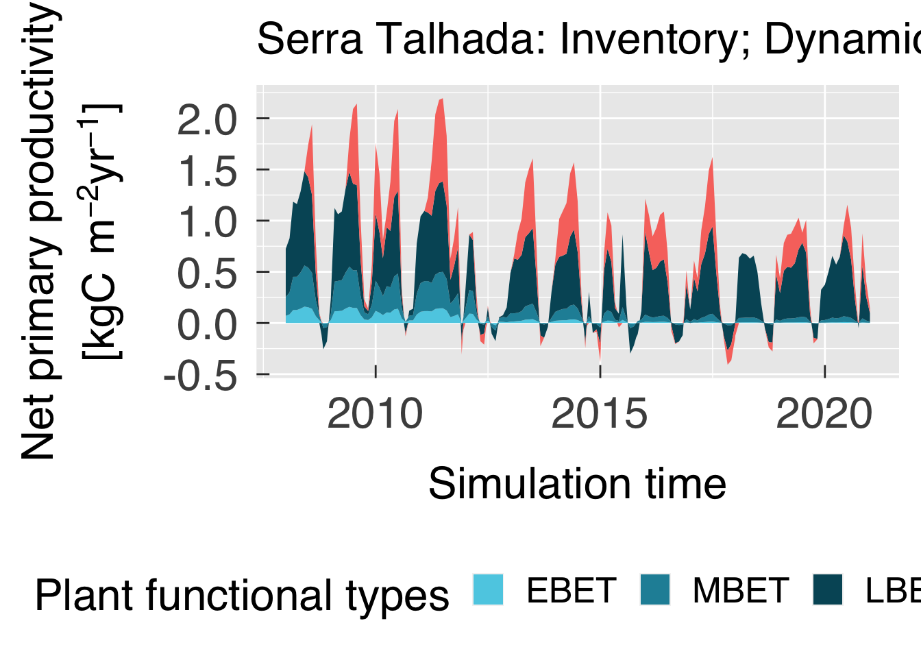
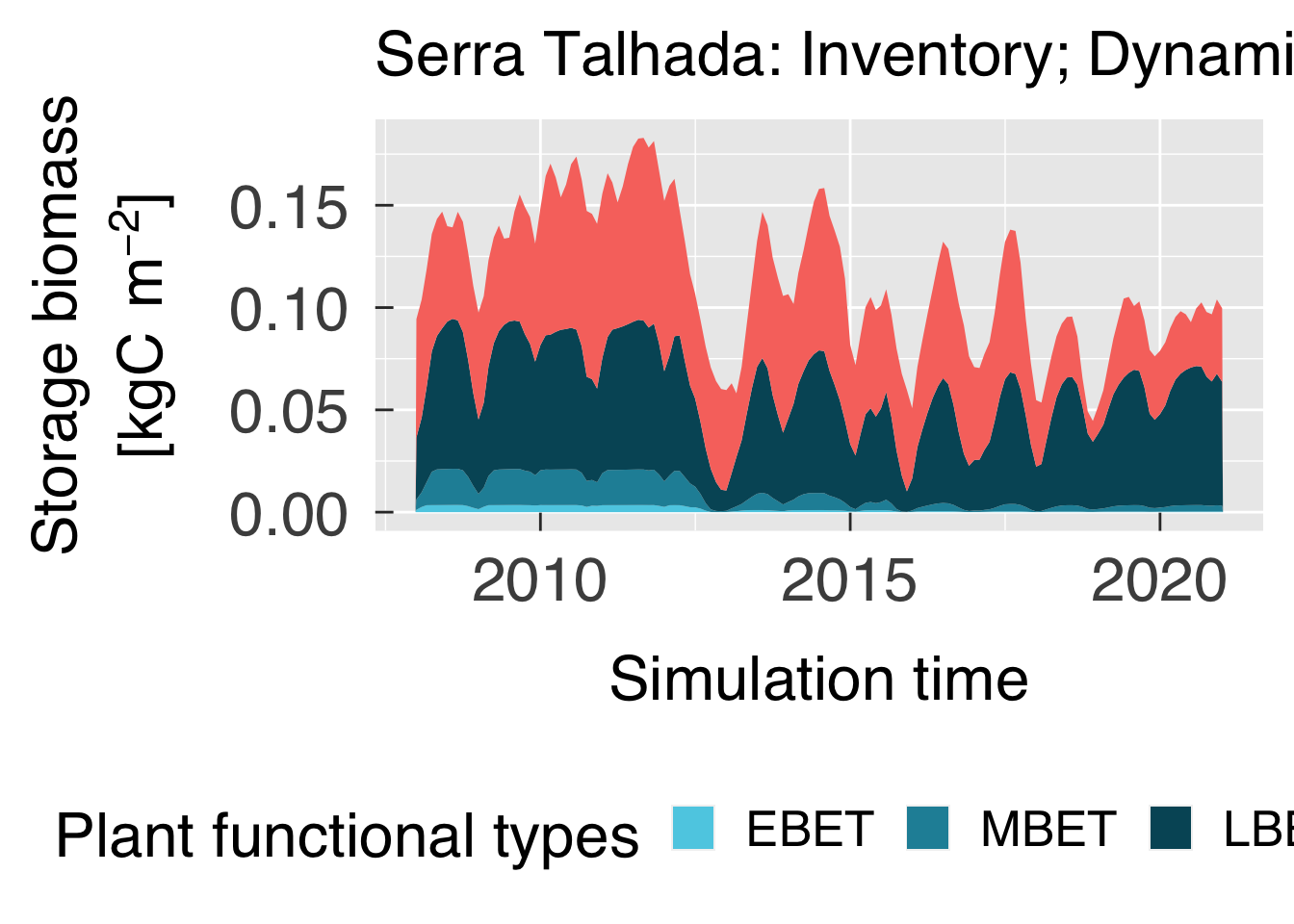
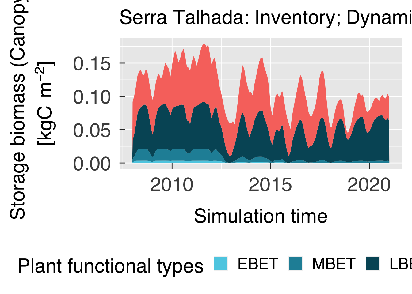
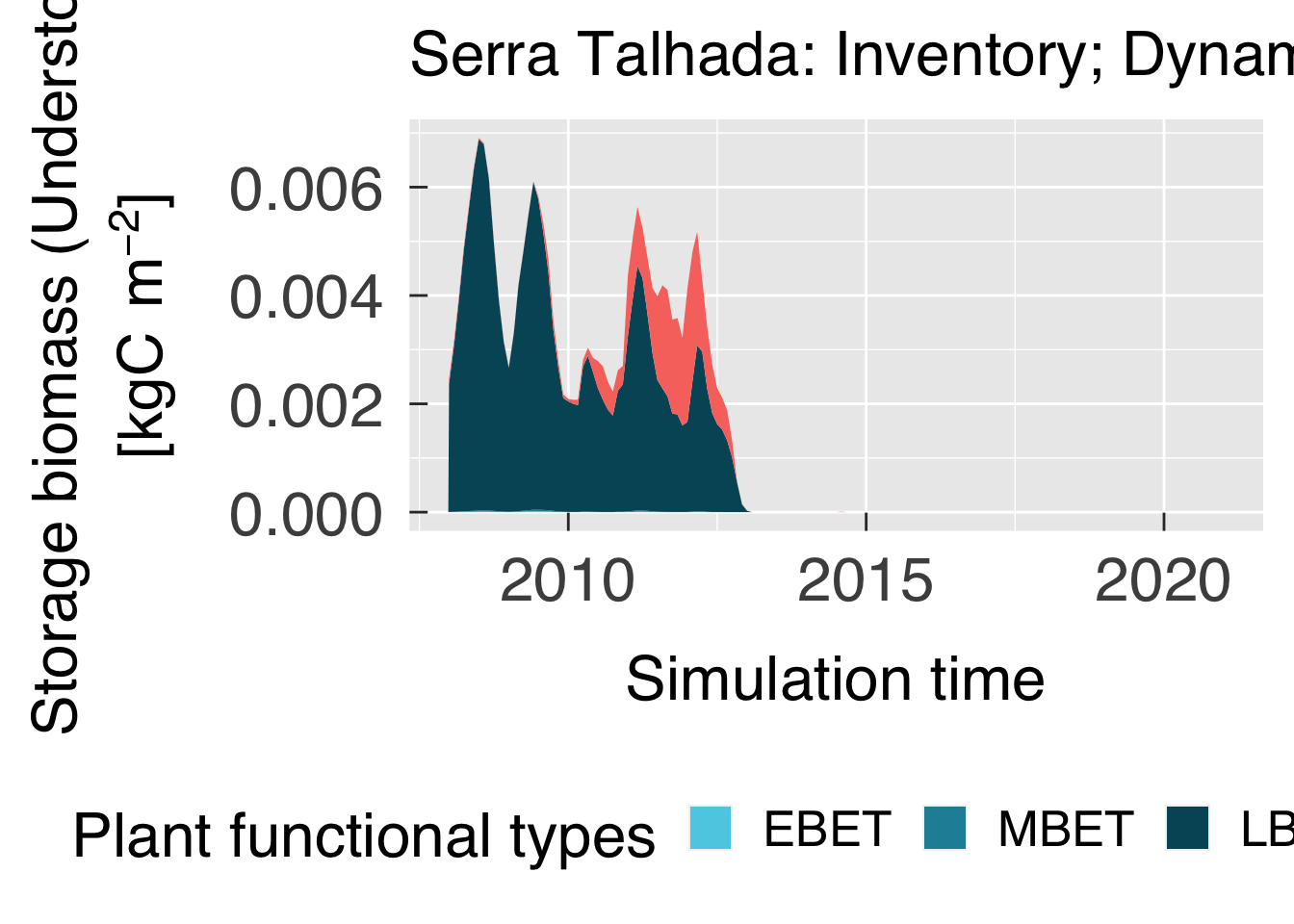
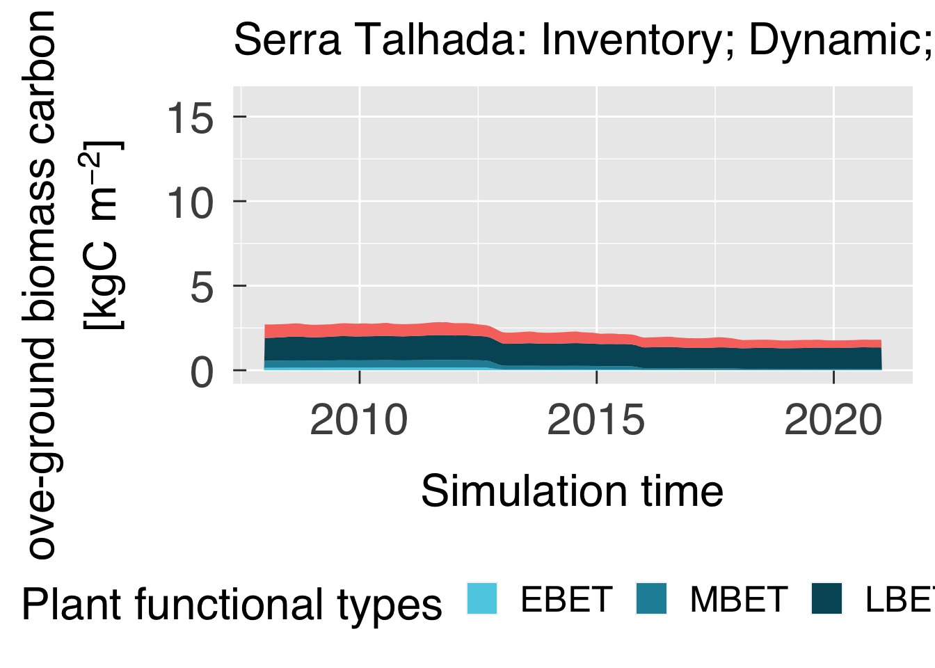
#---~---Plot time series by plant functional type:
cat0(" + Plot time series of size-dependent variables.")

# Title for legend
pft_legend = "Plant functional types"

pft_loop = which(fatesvar$vnam %in% names(bypft))
gg_pft   = list()
for (f in pft_loop){
  # Match variables.
  f_vnam   = fatesvar$vnam  [f]
  f_desc   = fatesvar$desc  [f]
  f_unit   = fatesvar$unit  [f]
  f_stack  = fatesvar$stack [f]
  f_ylower = fatesvar$ylower[f]
  f_yupper = fatesvar$yupper[f]
  cat0("   - ",f_desc,".")

  # Set plotting characteristics.
  f_bypft     = bypft
  f_bypft$pft = factor(f_bypft$pft,levels=sequence(npfts))
  f_colpfts   = pftinfo$colour
  f_pftlabs   = pftinfo$short

  # Initialise plot (decide whether to plot lines or stacks).
  if (f_stack){
     gg_now = ggplot(data=f_bypft,aes_string(x="time",y=f_vnam,group="pft",fill="pft"))
     gg_now = gg_now + scale_fill_manual(name=pft_legend,labels=f_pftlabs,values=f_colpfts)
     gg_now = gg_now + geom_area(position=position_stack(reverse = TRUE),show.legend = TRUE)
  }else{
     gg_now = ggplot(data=f_bypft,aes_string(x="time",y=f_vnam,group="pft",colour="pft"))
     gg_now = gg_now + scale_colour_manual(name=pft_legend,labels=f_pftlabs,values=f_colpfts)
     gg_now = gg_now + geom_line(lwd=1.0,show.legend = TRUE)
  }#end if (f_stack)
  gg_now = gg_now + labs(title=case_desc)
  gg_now = gg_now + scale_x_datetime(date_labels=gg_tfmt)
  if (all(is.finite(c(f_ylower,f_yupper)))){
     gg_now = gg_now + scale_y_continuous(limits=c(f_ylower,f_yupper),oob=oob_keep)
  }#end if (all(is.finite(f_ylower,f_yupper)))
  gg_now = gg_now + xlab("Simulation time")
  gg_now = gg_now + ylab(desc.unit(desc=f_desc,unit=untab[[f_unit]],twolines=TRUE))
  gg_now = gg_now + theme_grey( base_size = gg_ptsz, base_family = "Helvetica",base_line_size = 0.5,base_rect_size =0.5)
  gg_now = gg_now + theme( legend.position   = "bottom"
                         , axis.text.x       = element_text( size   = gg_ptsz
                                                           , margin = unit(rep(0.35,times=4),"cm")
                                                           )#end element_text
                         , axis.text.y       = element_text( size   = gg_ptsz
                                                           , margin = unit(rep(0.35,times=4),"cm")
                                                           )#end element_text
                         , plot.title        = element_text( size = gg_ptsz)
                         , axis.ticks.length = unit(-0.25,"cm")
                         )#end theme

  # Save plot in every format requested.
  for (d in sequence(ndevice)){
    f_output = paste0(f_vnam,"-tspft-",case_fpref,".",gg_device[d])
    dummy = ggsave( filename = f_output
                  , plot     = gg_now
                  , device   = gg_device[d]
                  , path     = tspft_path
                  , width    = gg_width
                  , height   = gg_height
                  , units    = gg_units
                  , dpi      = gg_depth
                  )#end ggsave
  }#end for (o in sequence(nout))

  # Write plot settings to the list.
  gg_pft[[f_vnam]] = gg_now
}#end for (f in pft_loop)


# If sought, plot images on screen
if (gg_screen) gg_pft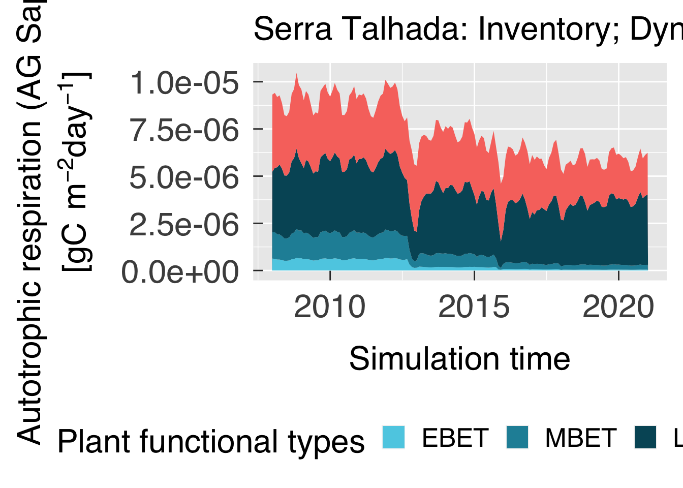
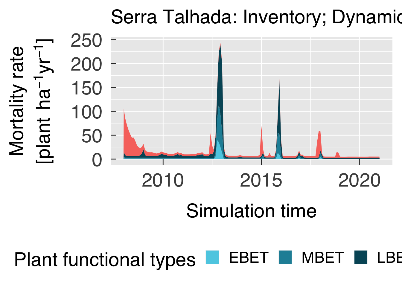
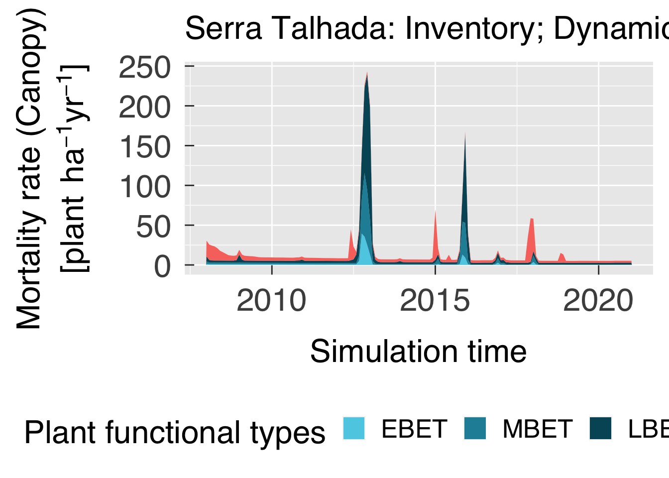
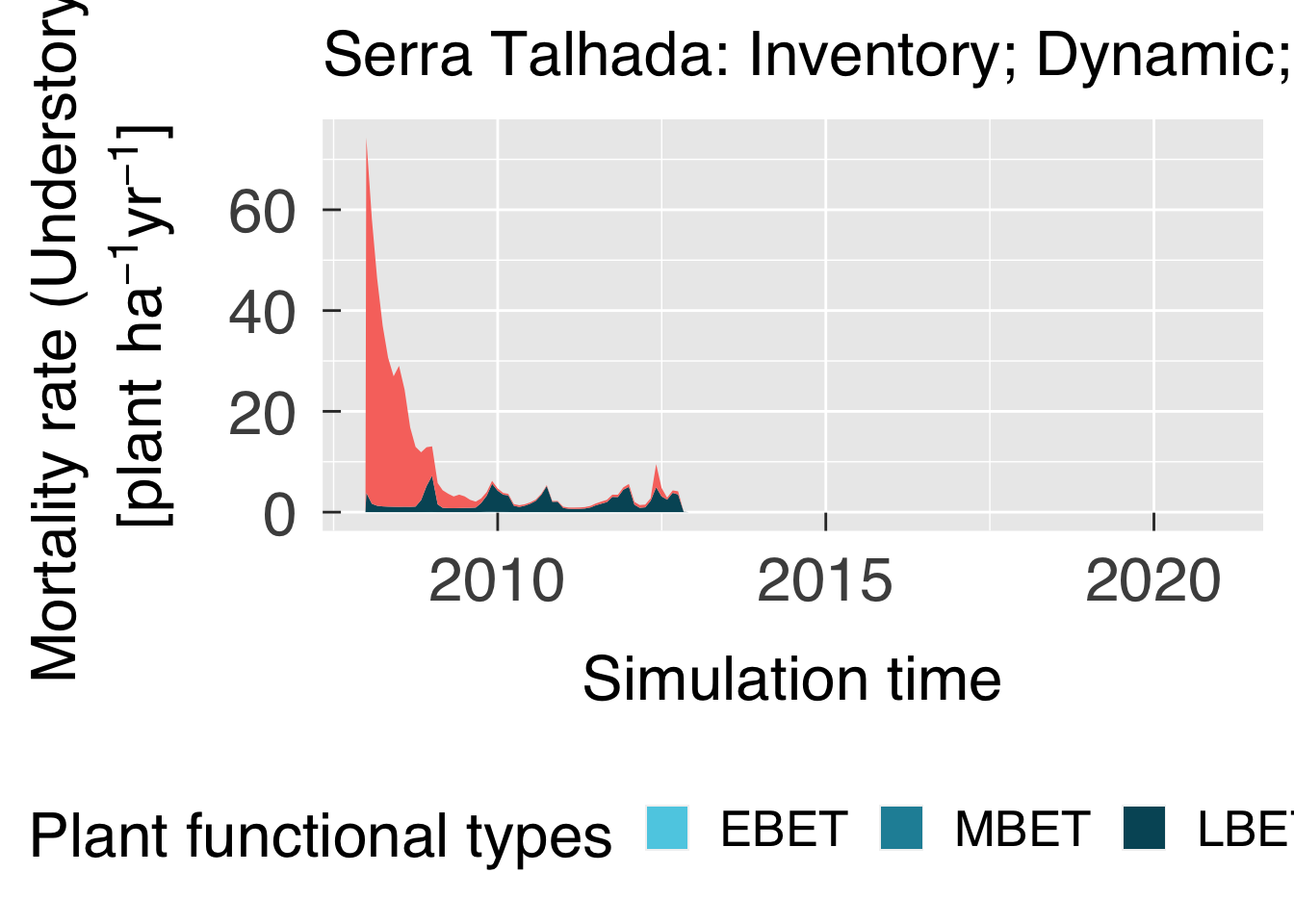
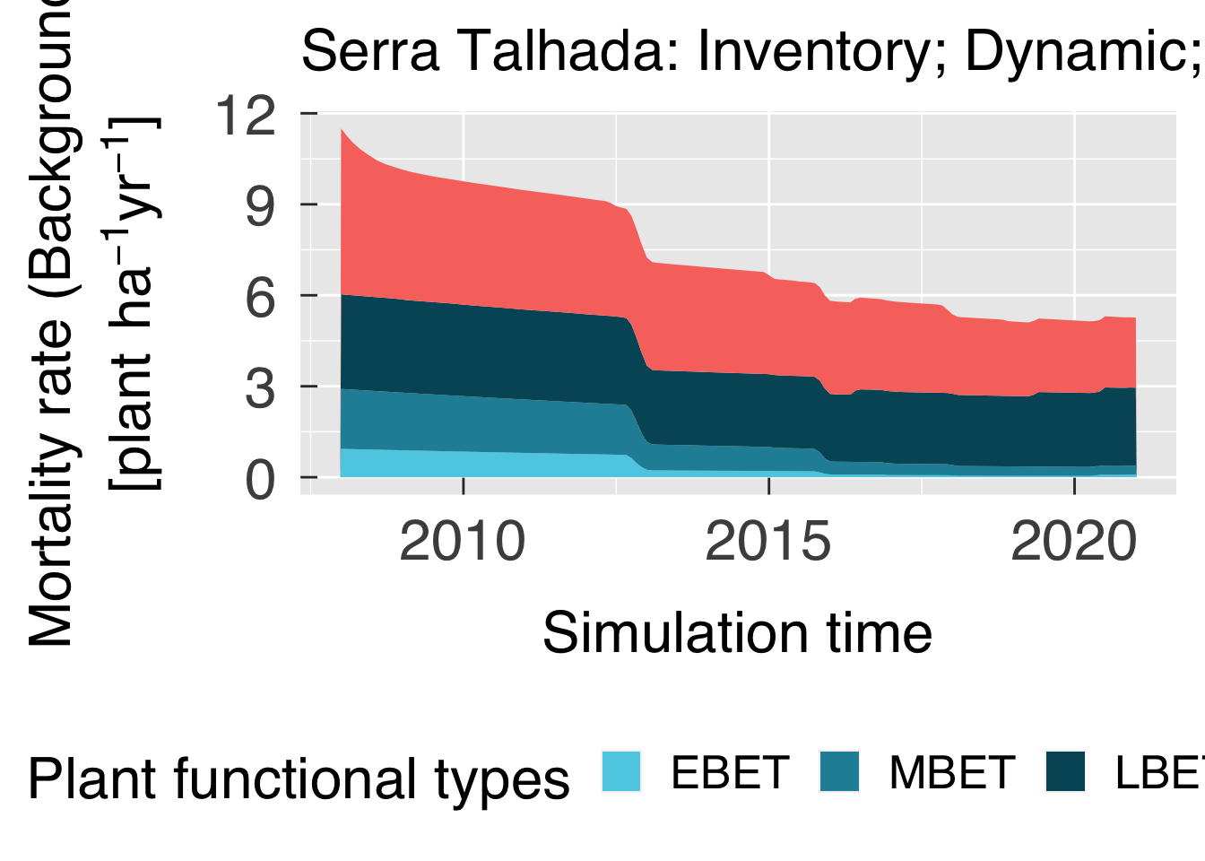
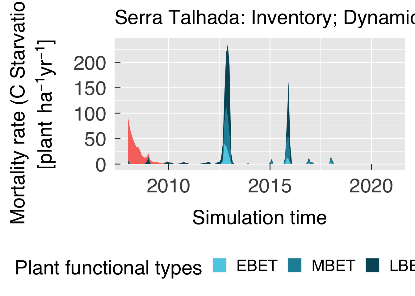

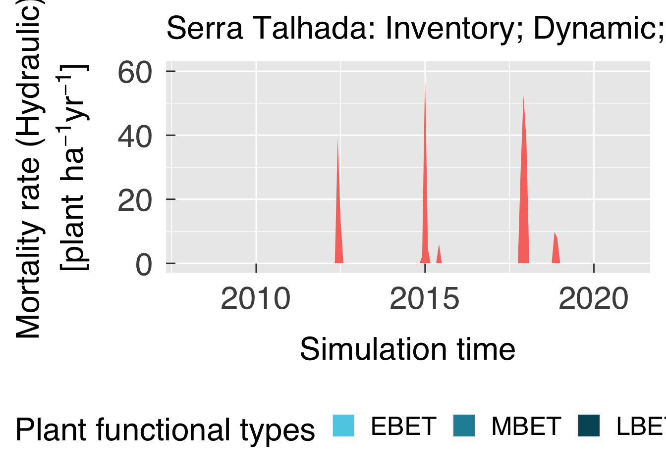
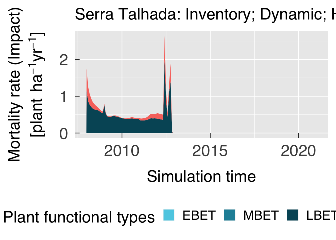
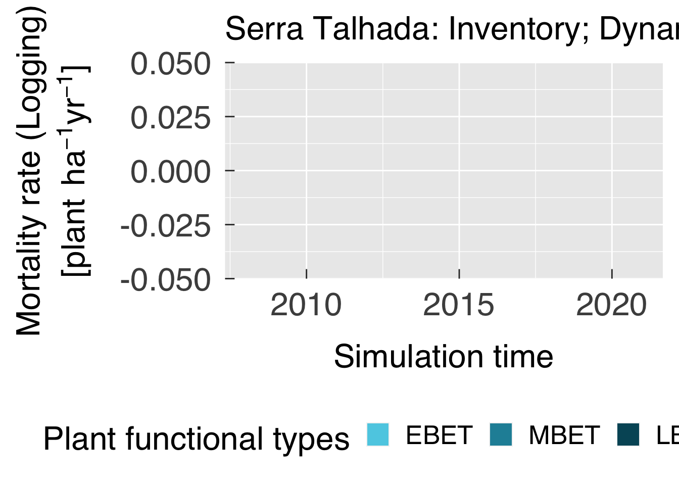
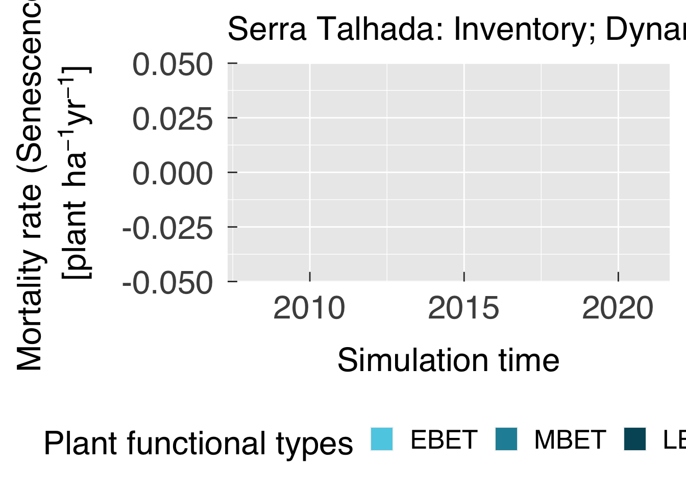
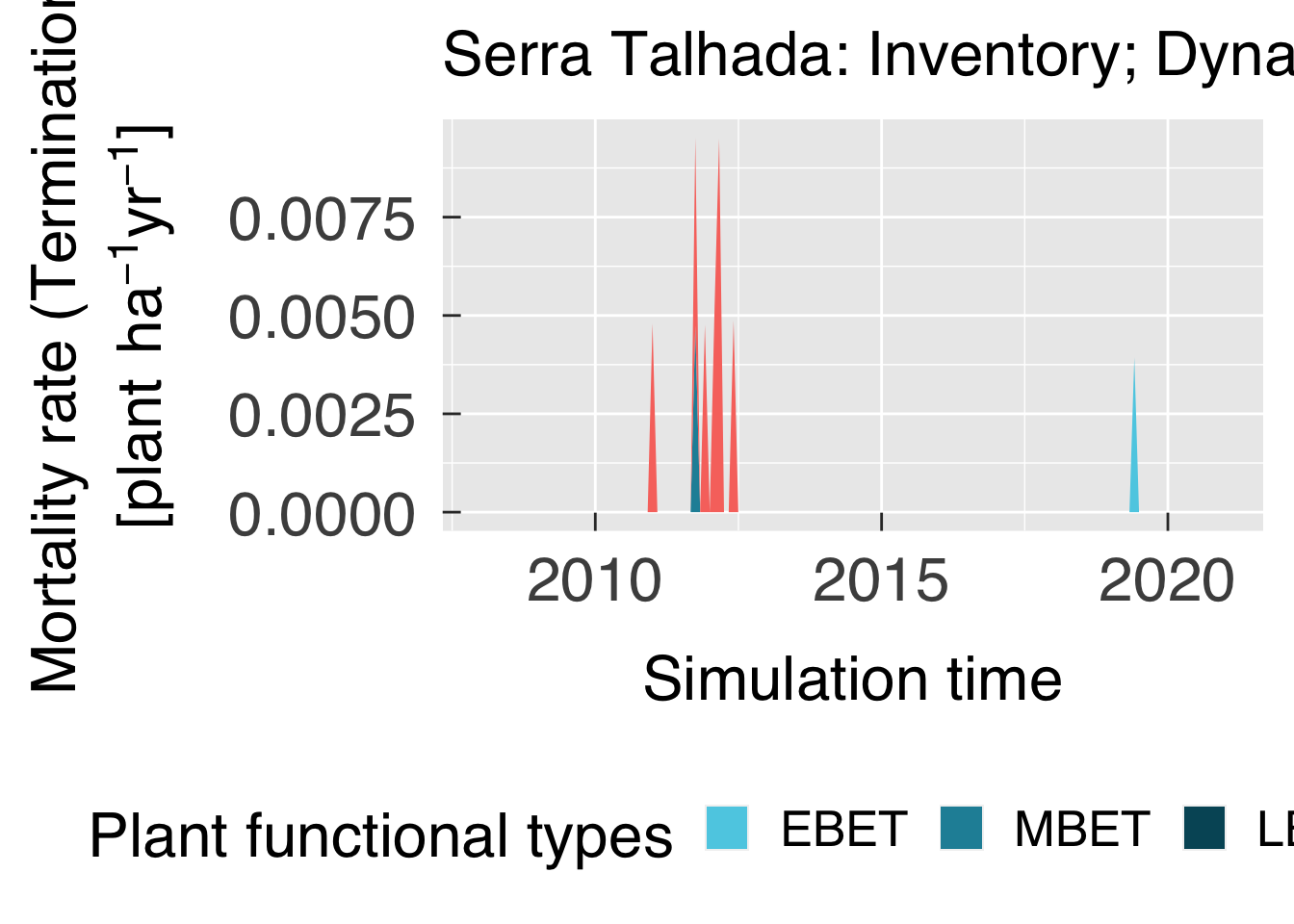
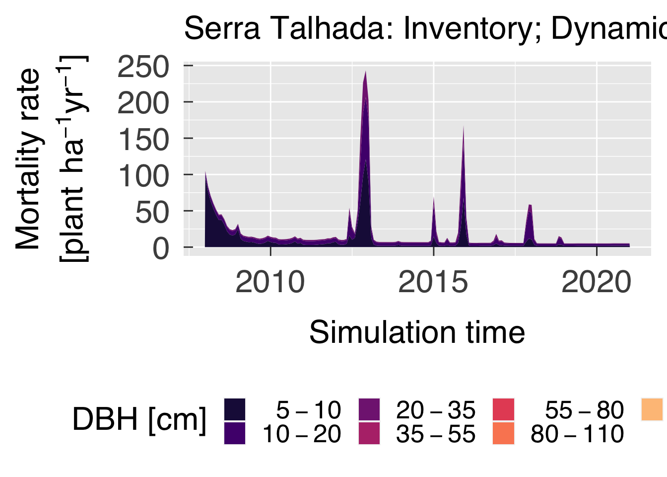
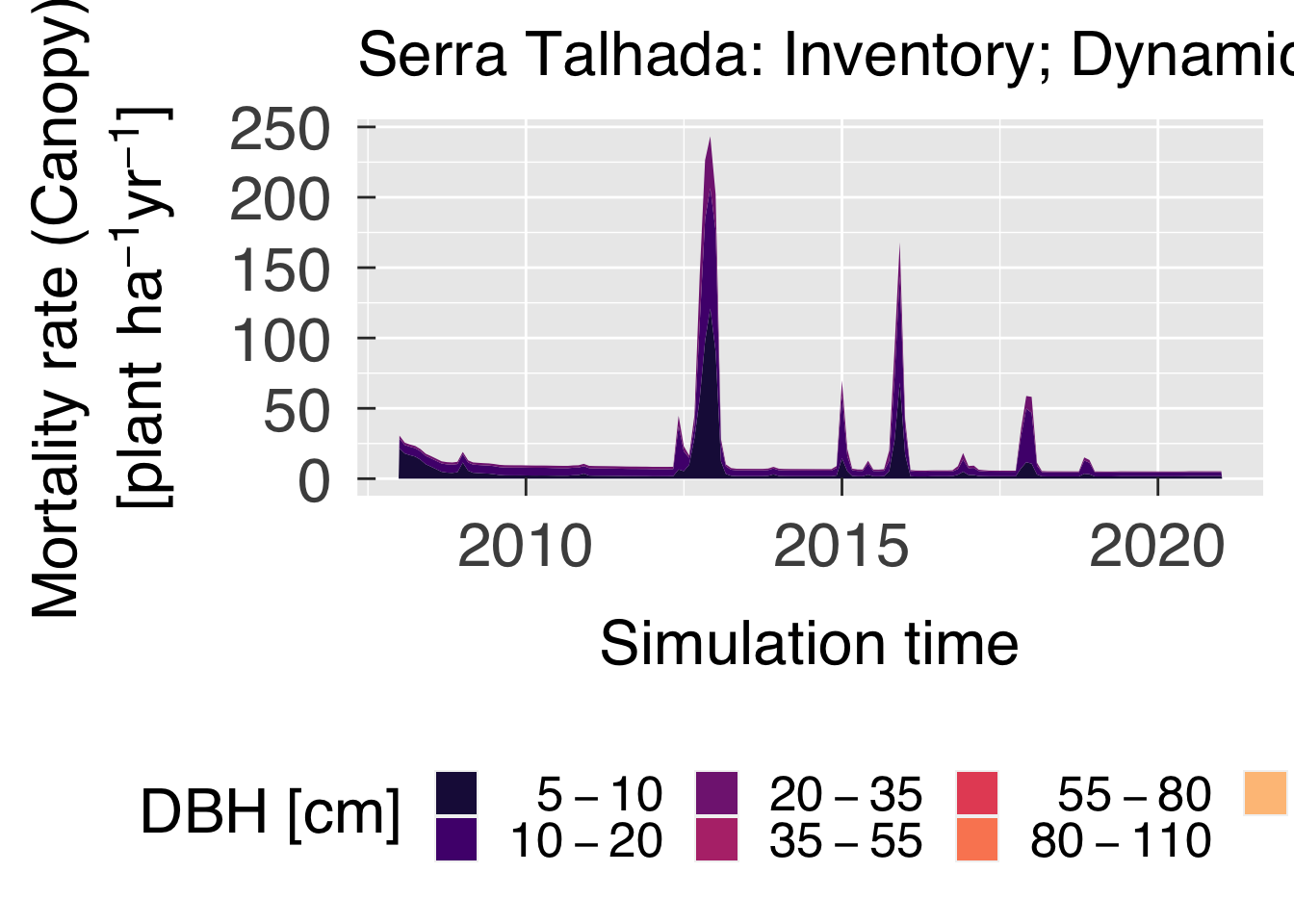
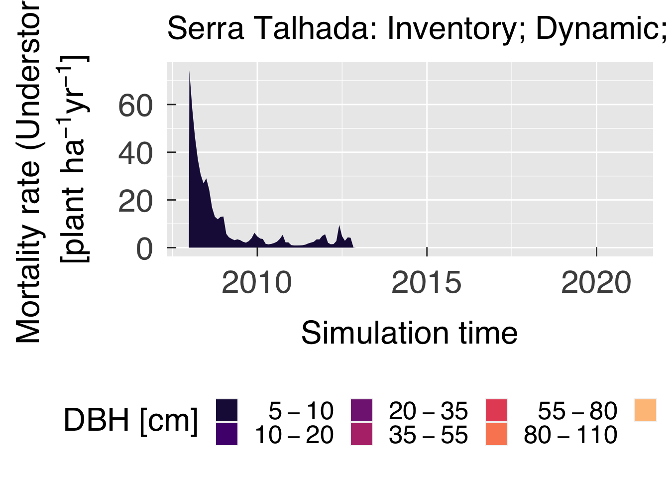
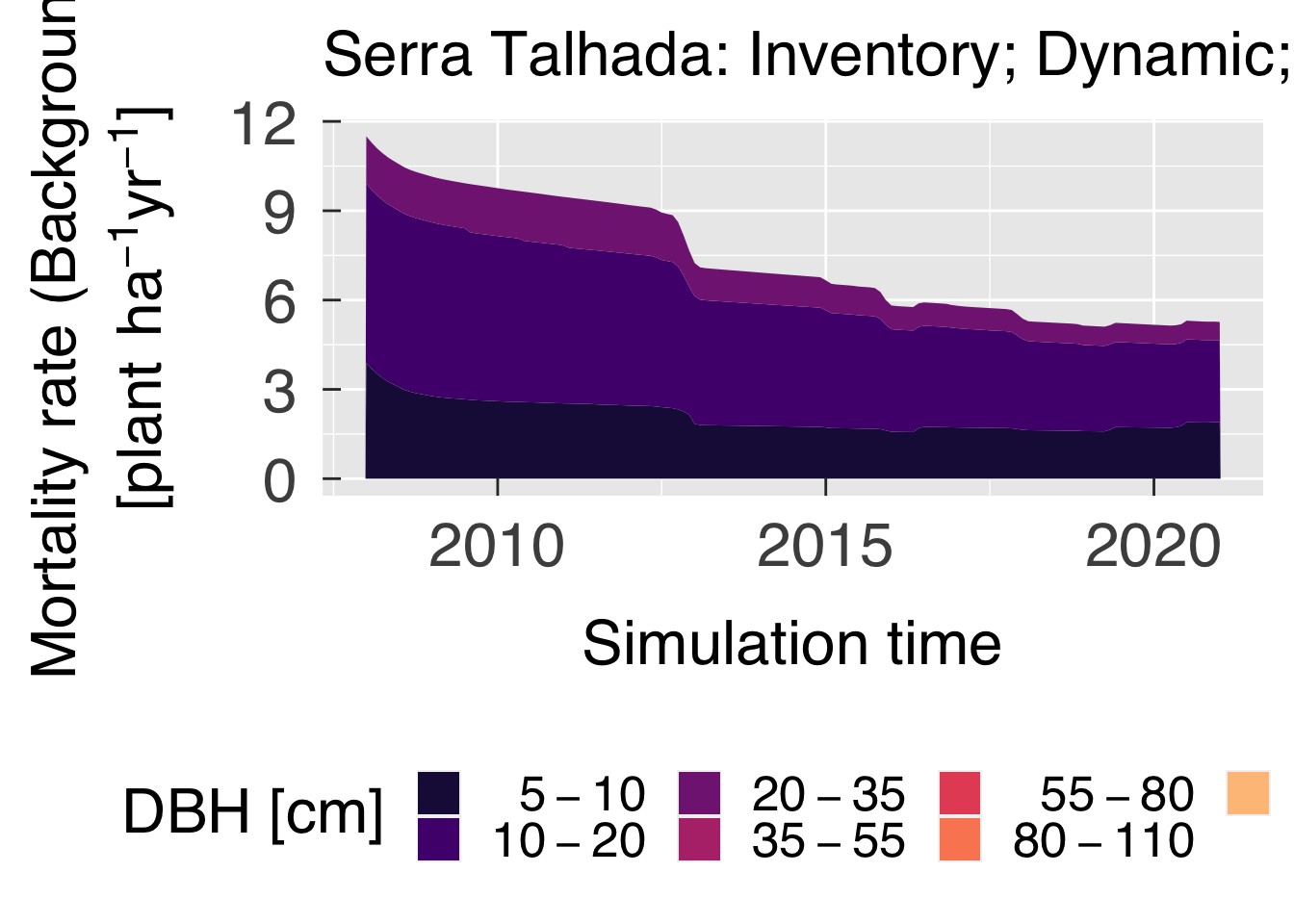
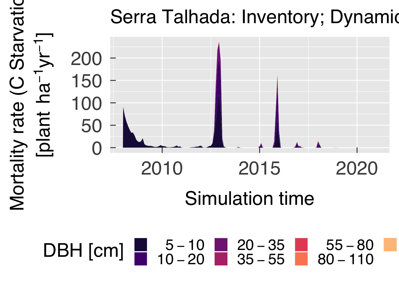
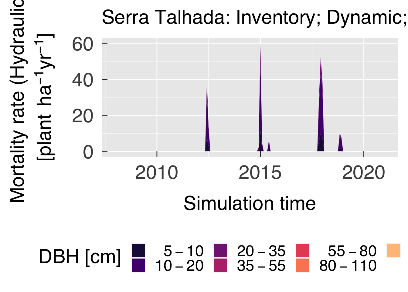
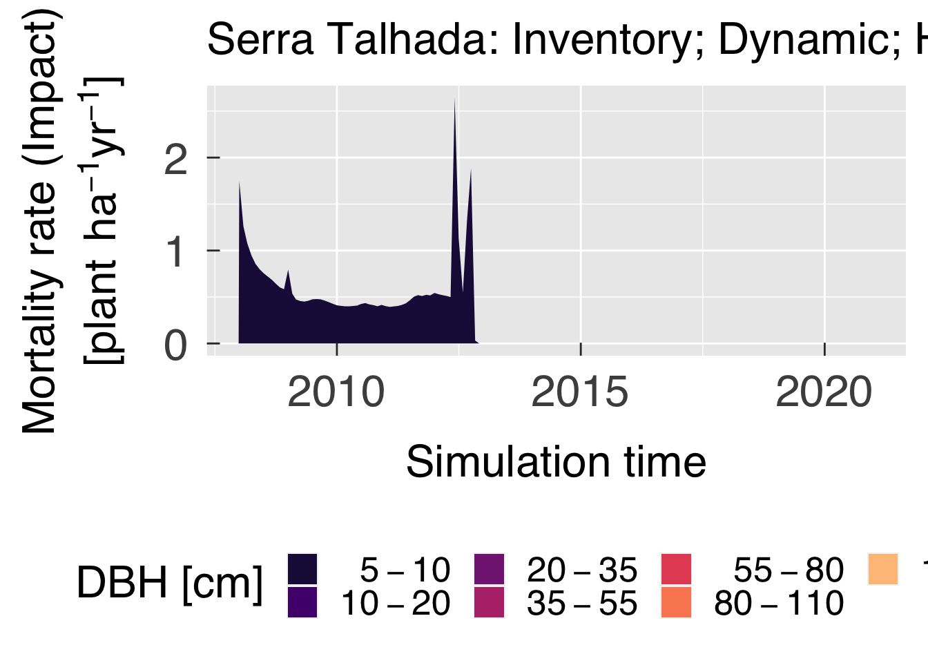
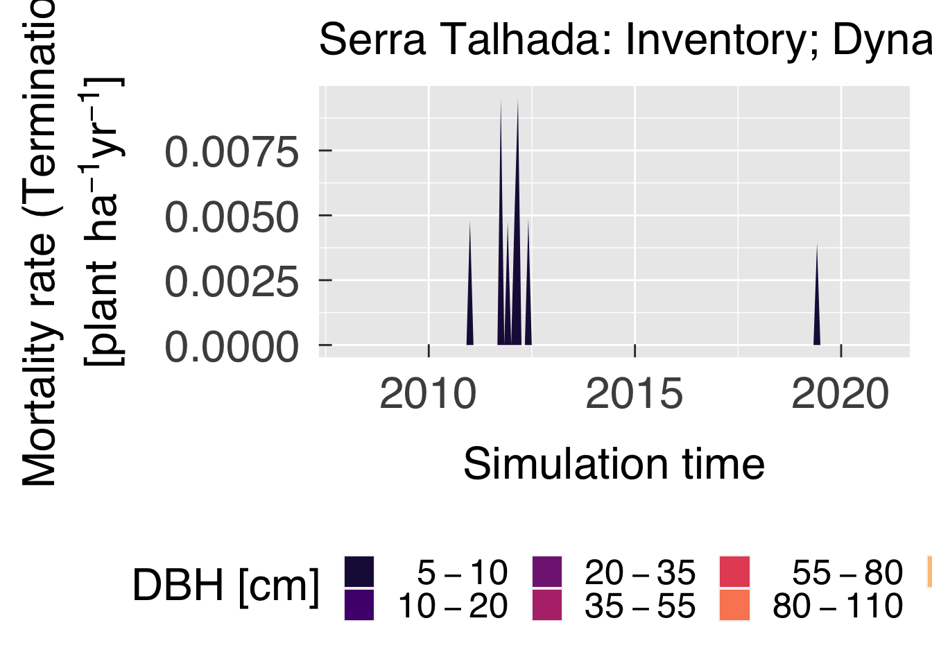
Plot time series by mortality type (multiple panels by PFT or by size/DBH class). Because all the mortality rates refer to the same baseline population, we convert the mortality from absolute scale to relative, which may be more informative.
Mortality rates are not directly comparable when calculated across different scales Sheil and May 1996, so to make the relative rate, we first compute the monthly mortality, and then extrapolate to yearly mortality (even though the mortality rate in FATES is reported in \(\mathrm{stems}\,\mathrm{ha}^{-1}\,\mathrm{yr}^{-1}\)).
# Select mortality type variables, ensure all of them are present.
mortvar        = fatesvar[fatesvar$vtype %in% "mort",]
mortvar        = mortvar[order(mortvar$order),,drop=FALSE]
mortvar$desc   = gsub(pattern="Mortality rate \\(",replacement="",x=mortvar$desc)
mortvar$desc   = gsub(pattern="\\)"               ,replacement="",x=mortvar$desc)
nmorts         = nrow(mortvar)
plot_mort_dbh  = all(c(mortvar$vnam,"fates_nplant") %in% names(bydbh))
plot_mort_pft  = all(c(mortvar$vnam,"fates_nplant") %in% names(bypft))

# Function to convert change rate into mortality rate, by accounting for the non-linearity across multiple time scales.
find_mort = function(x,n){
   # mort_mon = ifelse( test = n == 0, yes = 0., no = pmin(1.,x/n/12.))
   # mort_year = 100. * (1. - (1. - mort_mon)^12)
   mu        = ifelse( test = n == 0., yes = 0., no = 12*log((n+x/12.)/n) )
   mort_year = 100.* (1. - exp(-mu) )
   return(mort_year)
}#end function find_mort

# In case we are to plot mortality by type and PFT, reorganise mortality data.
if (plot_mort_pft){
   # Re-order mortality so it becomes all in one tibble.
   mortpft = bypft %>%
             mutate_at(all_of(mortvar$vnam), ~ find_mort(x=.x,n=.data$fates_nplant)) %>%
             select_at(all_of(c("time","pft",mortvar$vnam))) %>%
             pivot_longer(cols=mortvar$vnam,names_to="mtype",values_to="mortality") %>%
             mutate( mtype = factor(mortvar$desc[match(mtype,mortvar$vnam)],levels=mortvar$desc )
                   , pft   = factor(pftinfo$parse[match(pft,pftinfo$id)]   ,levels=pftinfo$parse) )


   # Initialise plot (decide whether to plot lines or stacks).
   gg_mpft = ggplot(data=mortpft,aes(x=time,y=mortality,group=mtype,fill=mtype))
   gg_mpft = gg_mpft + facet_wrap( ~ pft, ncol = 2, labeller = label_parsed)
   gg_mpft = gg_mpft + scale_fill_manual(name="Mortality type",labels=mortvar$desc,values=mortvar$colour)
   gg_mpft = gg_mpft + geom_area(position=position_stack(reverse = FALSE),show.legend = TRUE)
   gg_mpft = gg_mpft + labs(title=case_desc)
   gg_mpft = gg_mpft + scale_x_datetime(date_labels=gg_tfmt)
   gg_mpft = gg_mpft + scale_y_continuous(trans="sqrt",n.breaks=10,labels=label_number_auto())
   gg_mpft = gg_mpft + xlab("Simulation time")
   gg_mpft = gg_mpft + ylab(desc.unit(desc="Mortality rate",unit=untab$pcoyr,twolines=TRUE))
   gg_mpft = gg_mpft + theme_grey( base_size = gg_ptsz, base_family = "Helvetica",base_line_size = 0.5,base_rect_size =0.5)
   gg_mpft = gg_mpft + theme( axis.text.x       = element_text( size   = gg_ptsz
                                                              , margin = unit(rep(0.35,times=4),"cm")
                                                              )#end element_text
                            , axis.text.y       = element_text( size   = gg_ptsz
                                                              , margin = unit(rep(0.35,times=4),"cm")
                                                              )#end element_text
                            , axis.ticks.length = unit(-0.25,"cm")
                            , legend.position   = "bottom"
                            , legend.direction  = "horizontal"
                            )#end theme

   # Save plots.
   for (d in sequence(ndevice)){
      m_output = paste0("mort-bypft-",case_fpref,".",gg_device[d])
      dummy    = ggsave( filename = m_output
                       , plot     = gg_mpft
                       , device   = gg_device[d]
                       , path     = tsmort_path
                       , width    = gg_width
                       , height   = gg_height
                       , units    = gg_units
                       , dpi      = gg_depth
                       )#end ggsave

   }#end for (d in sequence(ndevice))

   # If sought, plot images on screen
   if (gg_screen) gg_mpft

}#end if (plot_mort_pft)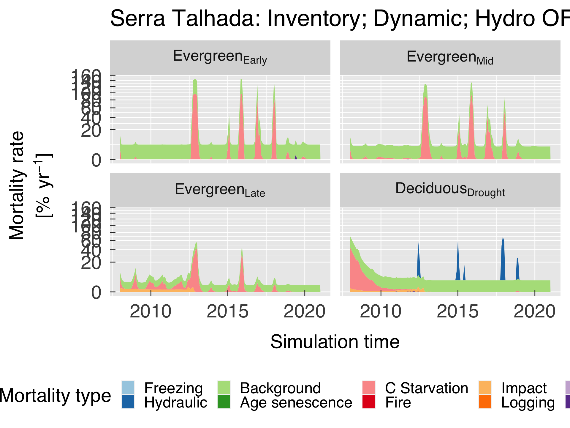
# In case we are to plot mortality by type and size(DBH), reorganise mortality data.
if (plot_mort_dbh){
   # Re-order mortality so it becomes all in one tibble.
   mortdbh = bydbh %>%
             filter( dbh != 1) %>%
             mutate_at(all_of(mortvar$vnam), ~ find_mort(x=.x,n=.data$fates_nplant)) %>%
             select_at(all_of(c("time","dbh",mortvar$vnam))) %>%
             pivot_longer(cols=mortvar$vnam,names_to="mtype",values_to="mortality") %>%
             mutate( mtype = factor(mortvar$desc[match(mtype,mortvar$vnam)],levels=mortvar$desc    )
                   , dbh   = factor(dbhinfo$desc[match(dbh  ,dbhinfo$id  )],levels=dbhinfo$desc[-1]) )

   # Initialise plot (decide whether to plot lines or stacks).
   gg_mdbh = ggplot(data=mortdbh,aes(x=time,y=mortality,group=mtype,fill=mtype))
   gg_mdbh = gg_mdbh + facet_wrap( ~ dbh, ncol = 3, labeller = label_parsed)
   gg_mdbh = gg_mdbh + scale_fill_manual(name="Mortality type",labels=mortvar$desc,values=mortvar$colour)
   gg_mdbh = gg_mdbh + geom_area(position=position_stack(reverse = FALSE),show.legend = TRUE)
   gg_mdbh = gg_mdbh + labs(title=case_desc)
   gg_mdbh = gg_mdbh + scale_x_datetime(date_labels=gg_tfmt)
   gg_mdbh = gg_mdbh + scale_y_continuous(trans="sqrt",n.breaks=10,labels=label_number_auto())
   gg_mdbh = gg_mdbh + xlab("Simulation time")
   gg_mdbh = gg_mdbh + ylab(desc.unit(desc="Mortality rate",unit=untab$pcoyr,twolines=TRUE))
   gg_mdbh = gg_mdbh + theme_grey( base_size = gg_ptsz, base_family = "Helvetica",base_line_size = 0.5,base_rect_size =0.5)
   gg_mdbh = gg_mdbh + theme( axis.text.x       = element_text( size   = gg_ptsz
                                                              , margin = unit(rep(0.35,times=4),"cm")
                                                              )#end element_text
                            , axis.text.y       = element_text( size   = gg_ptsz
                                                              , margin = unit(rep(0.35,times=4),"cm")
                                                              )#end element_text
                            , plot.title        = element_text( size = gg_ptsz)
                            , axis.ticks.length = unit(-0.25,"cm")
                            , legend.position   = "bottom"
                            , legend.direction  = "horizontal"
                            )#end theme

   # Save plots.
   for (d in sequence(ndevice)){
      m_output = paste0("mort-bydbh-",case_fpref,".",gg_device[d])
      dummy    = ggsave( filename = m_output
                       , plot     = gg_mdbh
                       , device   = gg_device[d]
                       , path     = tsmort_path
                       , width    = gg_width*2
                       , height   = gg_height*2
                       , units    = gg_units
                       , dpi      = gg_depth
                       )#end ggsave

   }#end for (d in sequence(ndevice))

   # If sought, plot images on screen
   if (gg_screen) gg_mdbh

}#end if (plot_mort_dbh)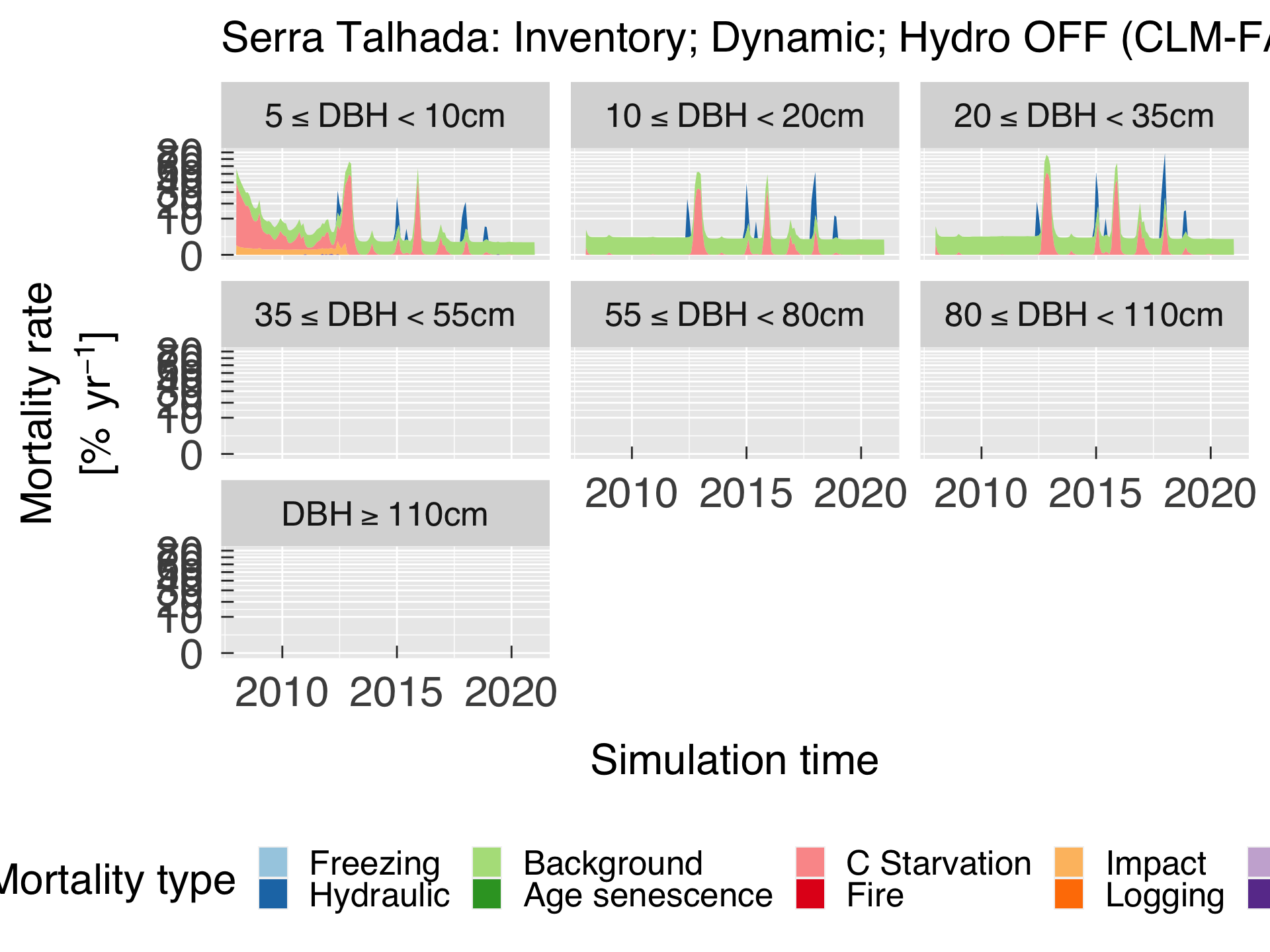
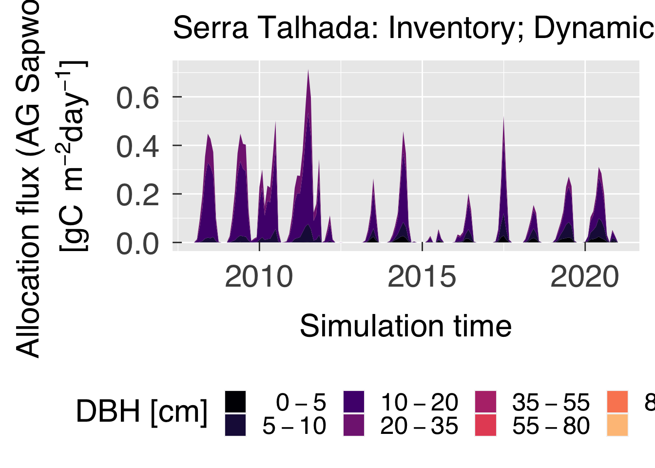
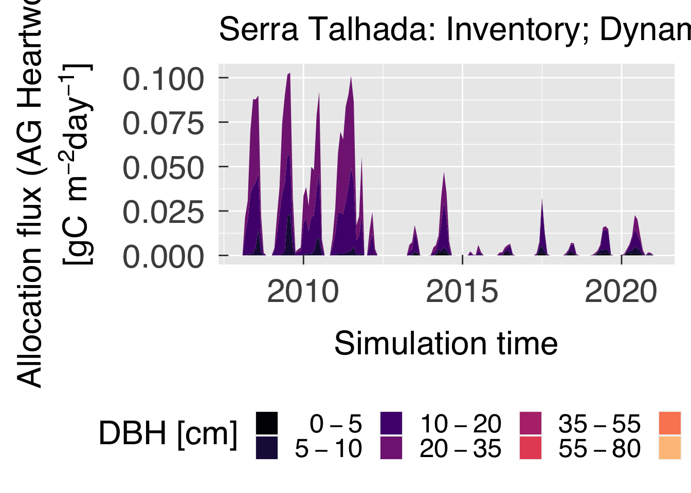
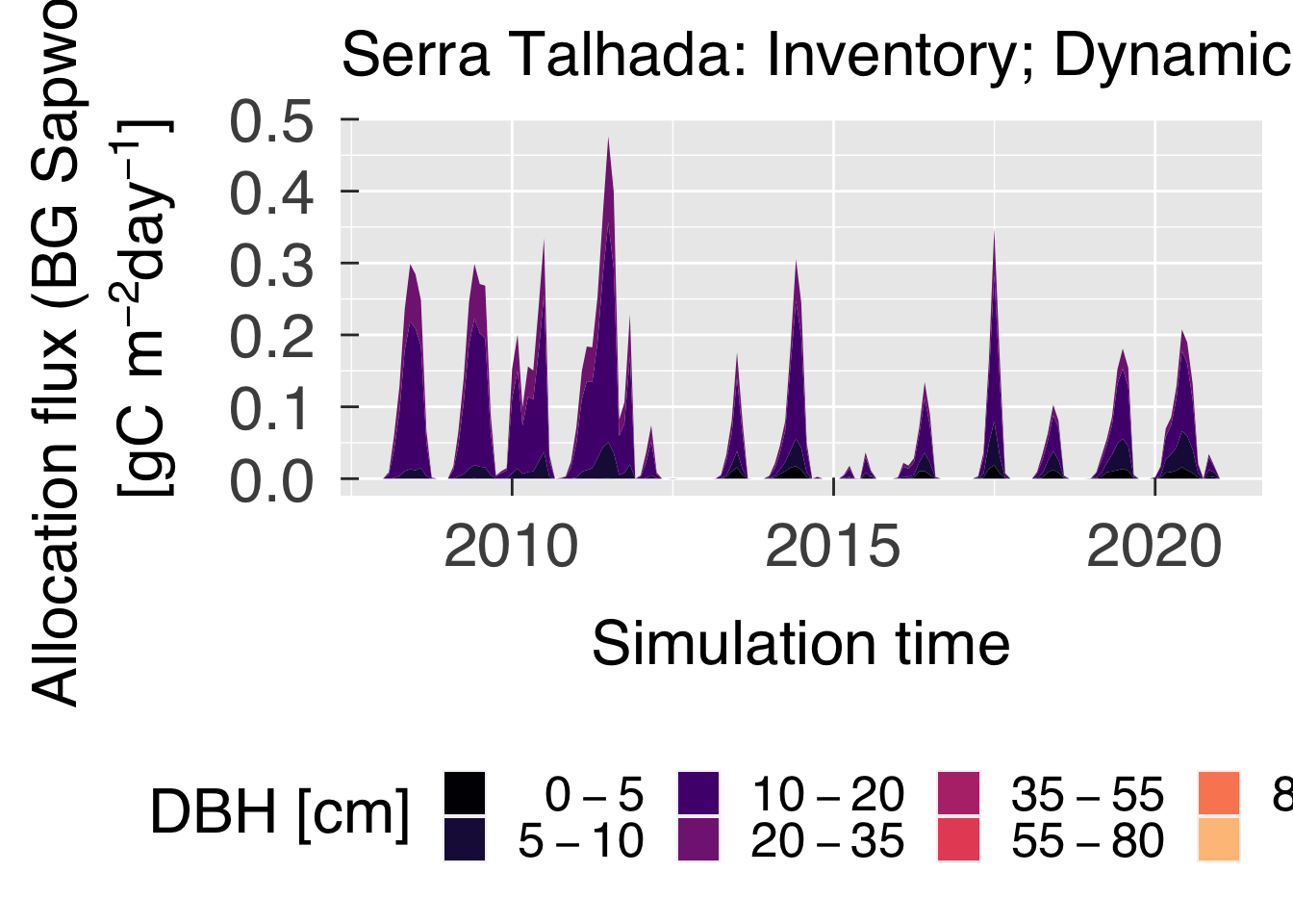
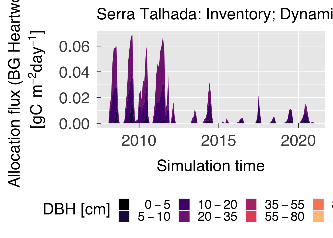
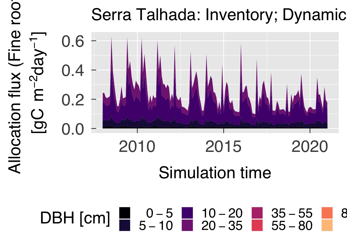
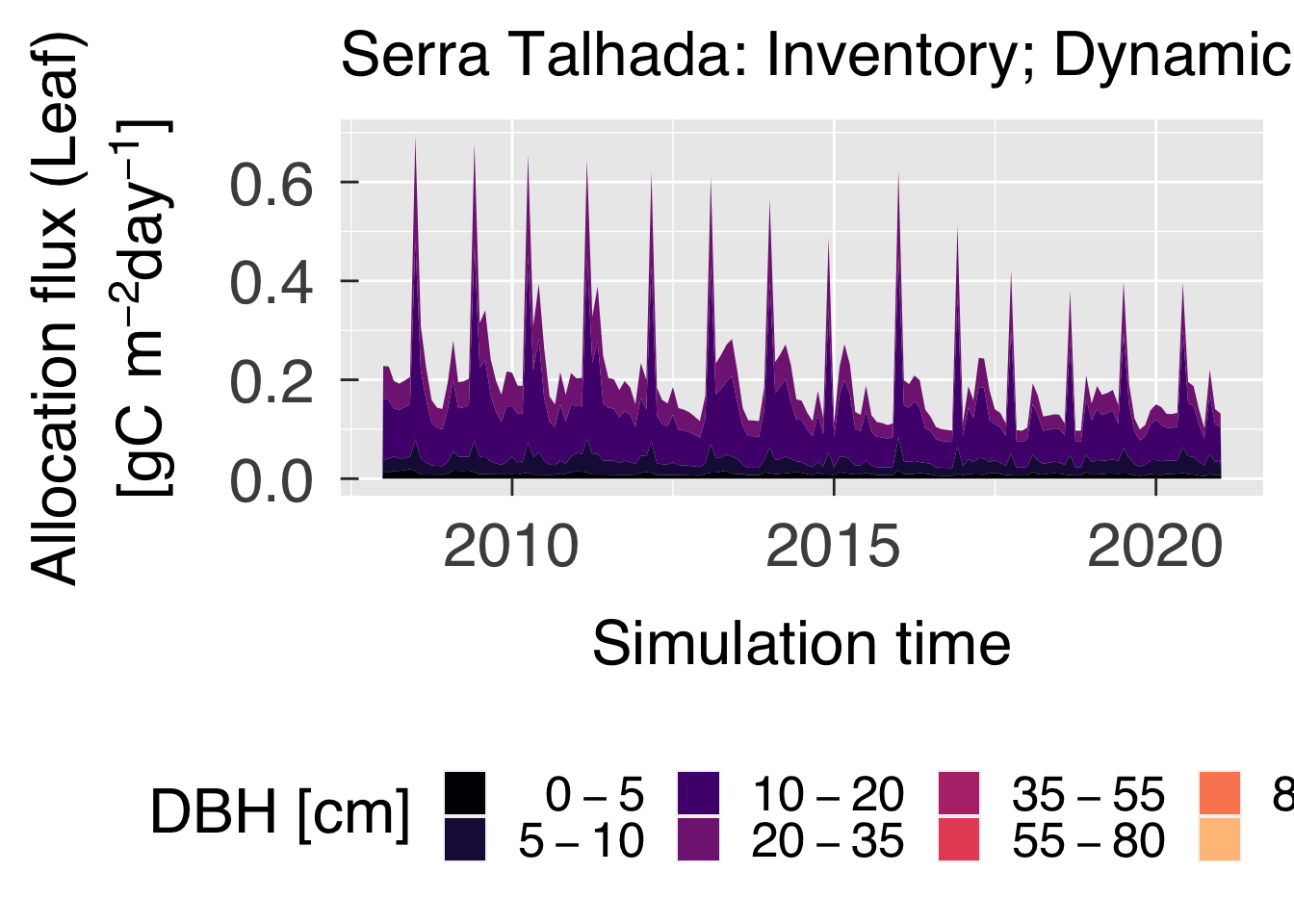
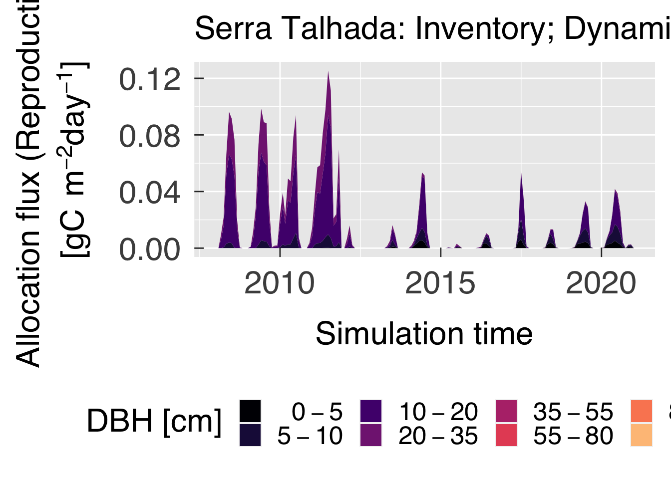
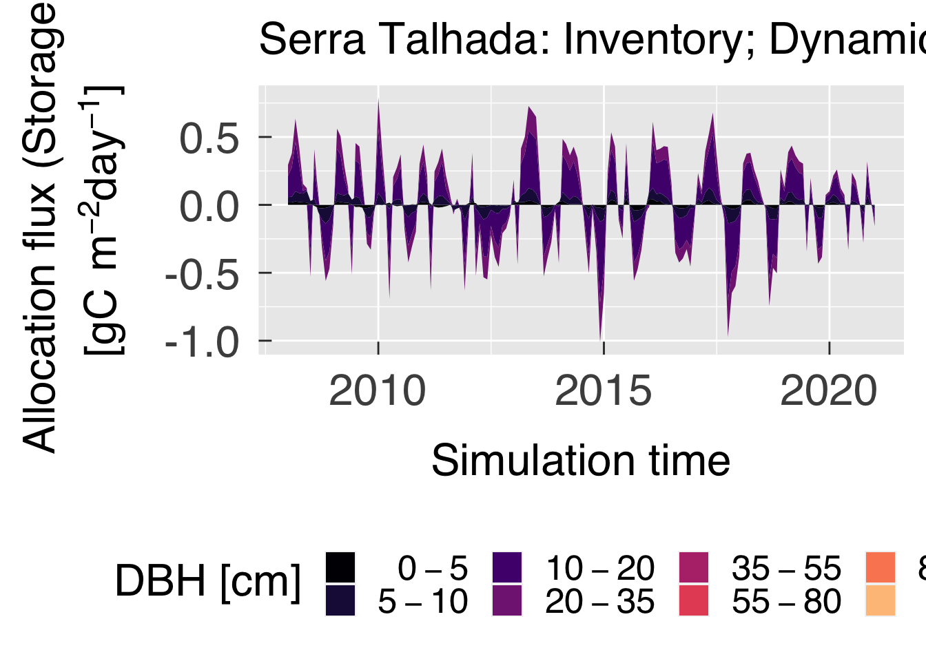
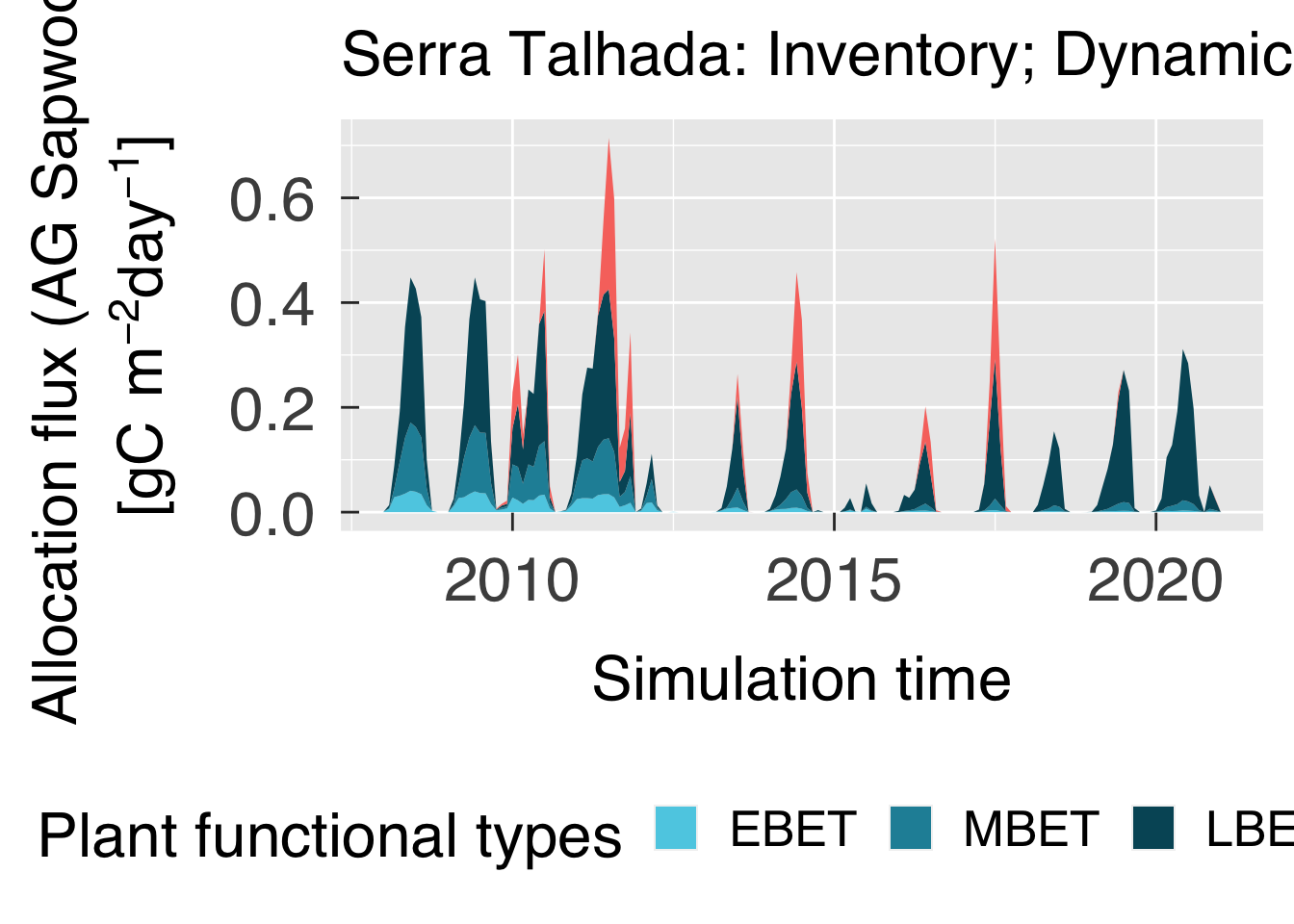
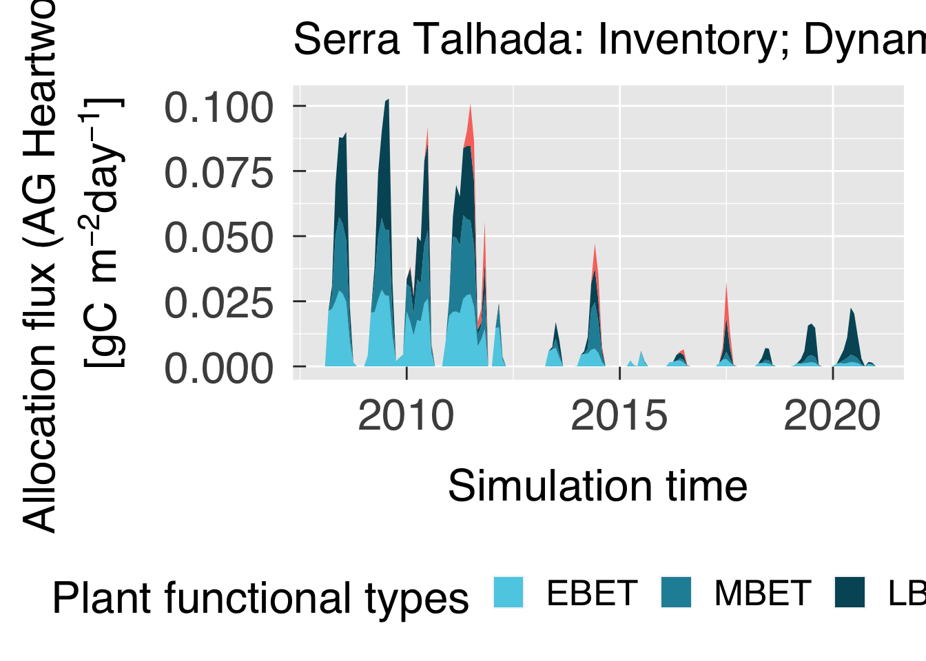
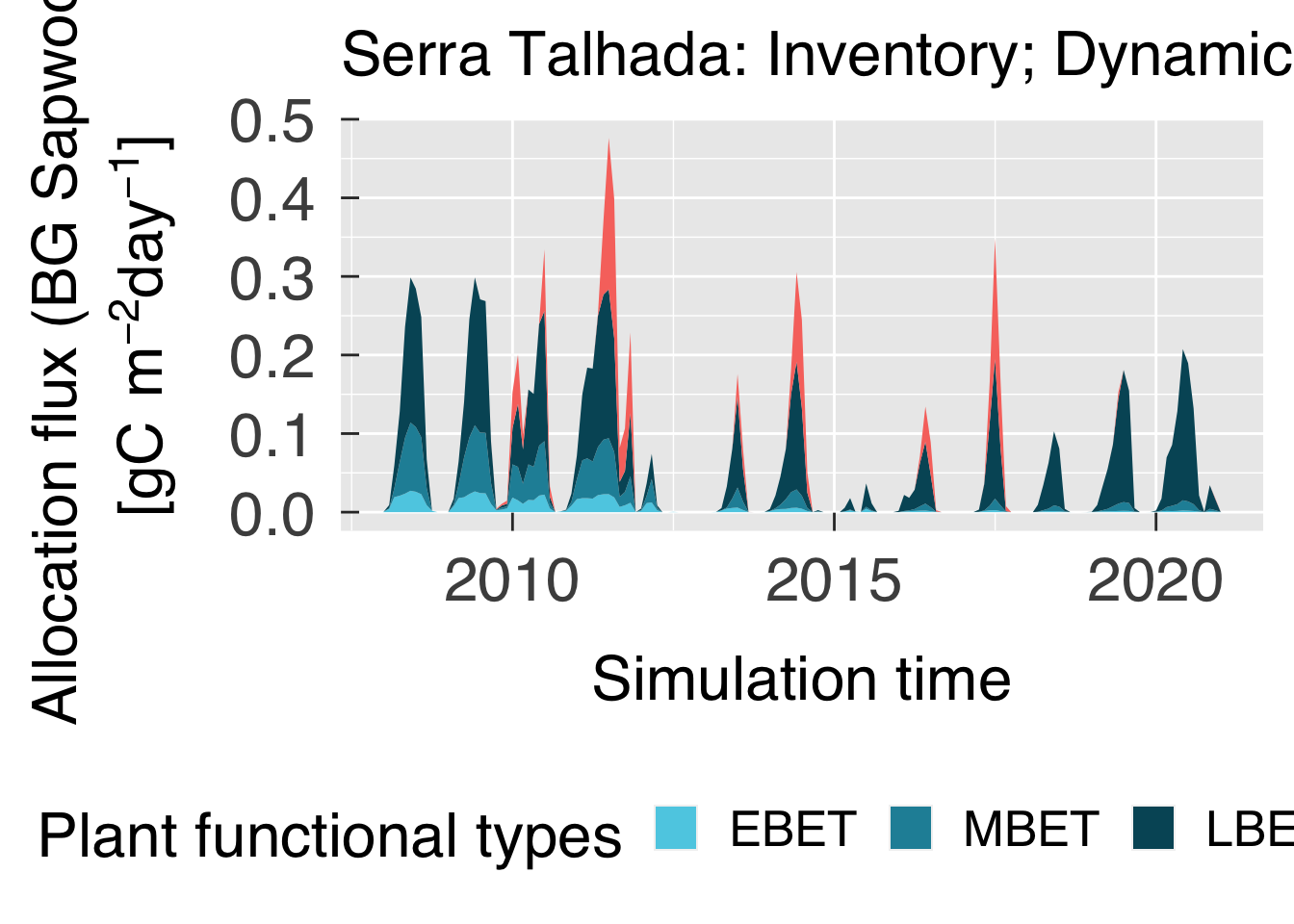
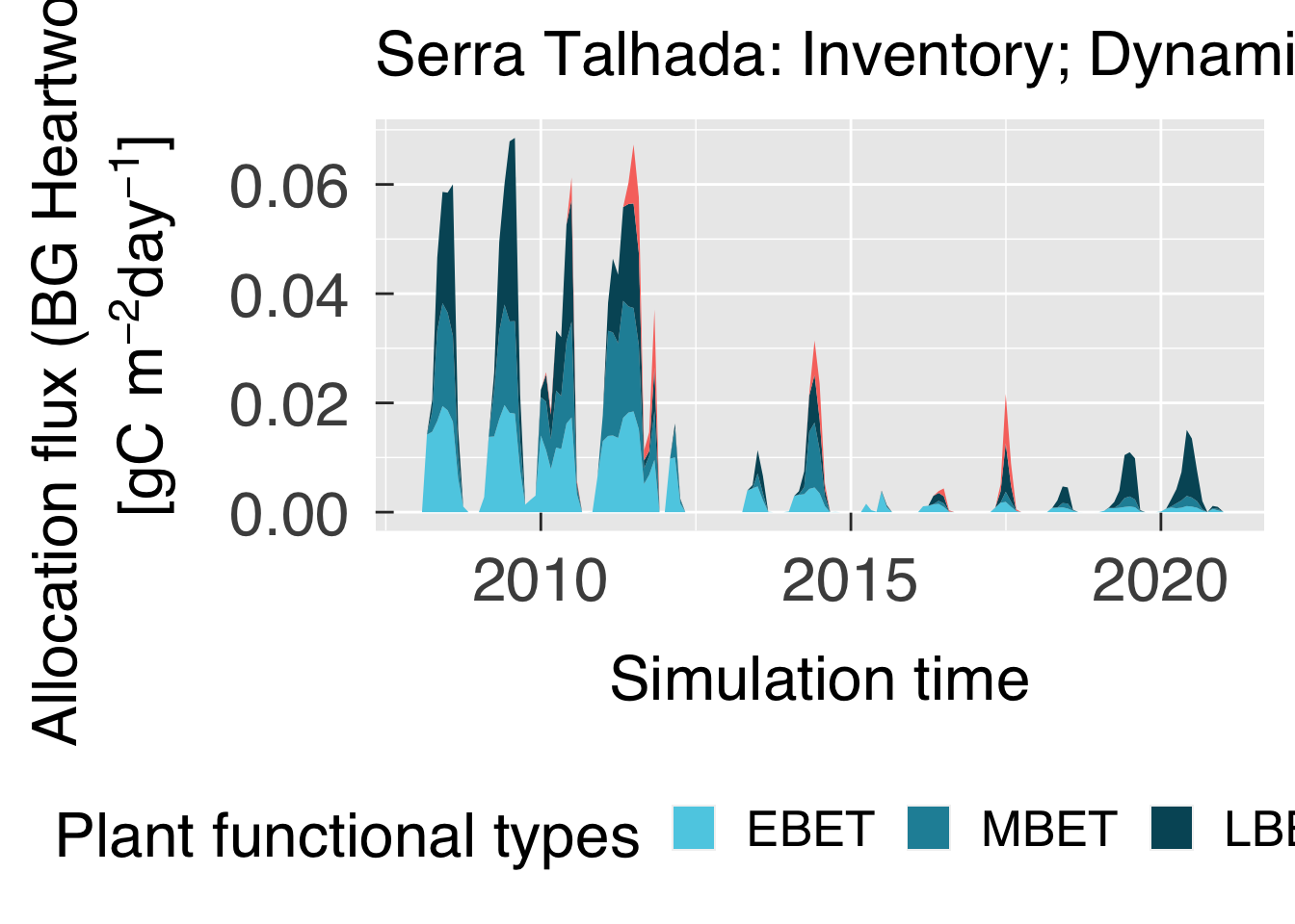
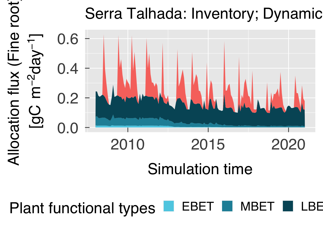
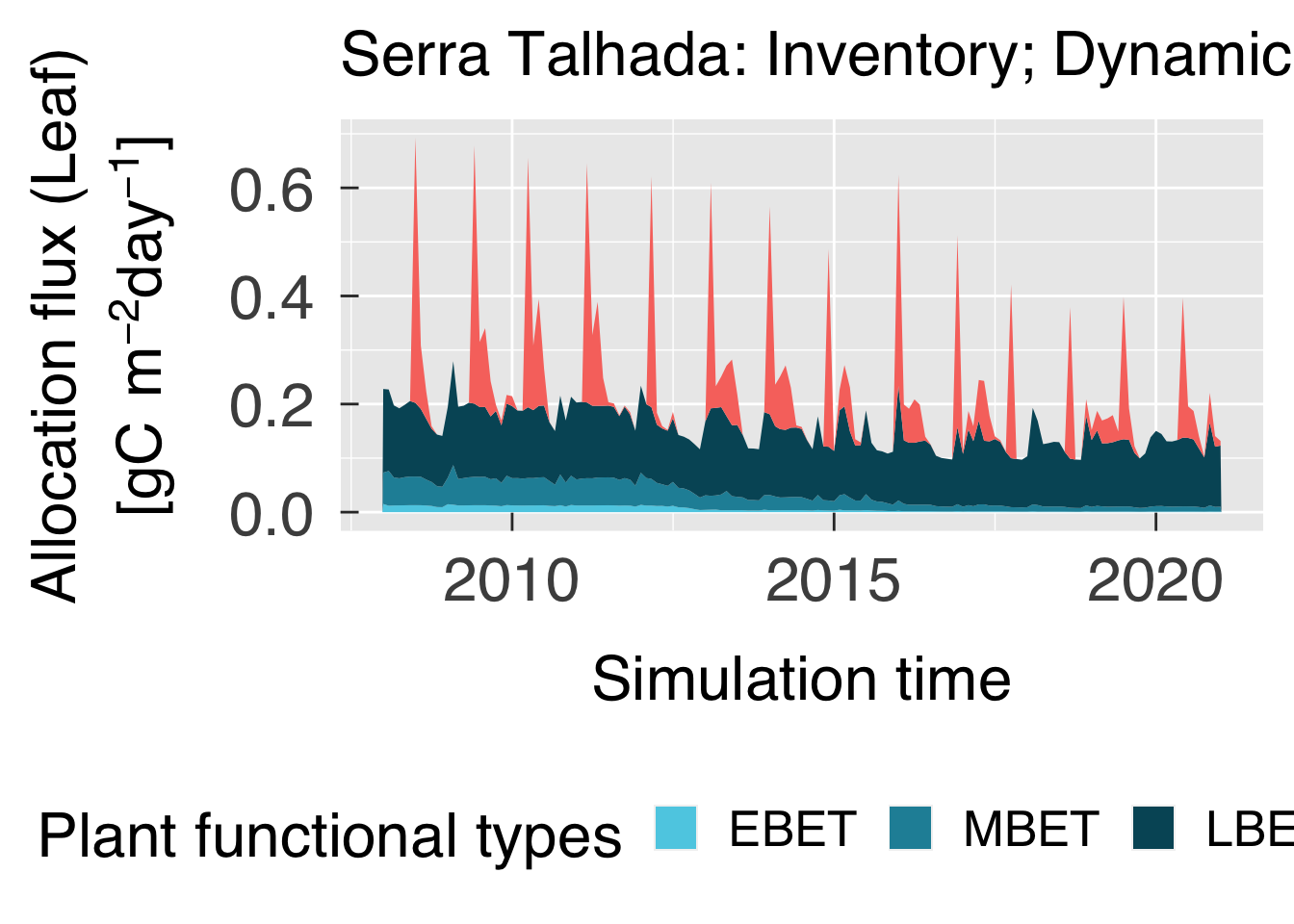
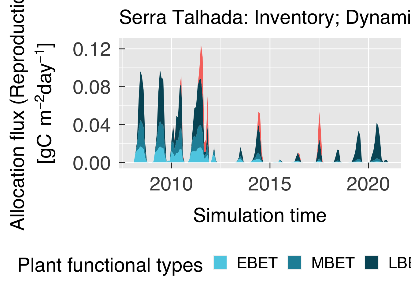
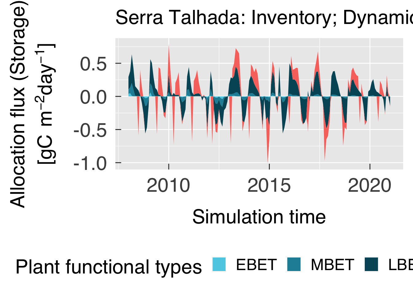
Plot time series of allocation by organ type (multiple panels by PFT or by size/DBH class).
# Select mortality type variables, ensure all of them are present.
allocvar        = fatesvar[fatesvar$vtype %in% "alloc",]
allocvar        = allocvar[order(allocvar$order),,drop=FALSE]
allocvar$desc   = gsub(pattern="Allocation flux \\(",replacement="",x=allocvar$desc)
allocvar$desc   = gsub(pattern="\\)"         ,replacement="",x=allocvar$desc)
nallocs         = nrow(allocvar)
plot_alloc_dbh  = all(allocvar$vnam %in% names(bydbh))
plot_alloc_pft  = all(allocvar$vnam %in% names(bypft))

# In case we are to plot NPP by type and PFT, reorganise NPP data.
if (plot_alloc_pft){
   # Re-order NPP so it becomes all in one tibble.
   allocpft = bypft %>%
      select_at(all_of(c("time","pft",allocvar$vnam))) %>%
      pivot_longer(cols=allocvar$vnam,names_to="otype",values_to="npp") %>%
      mutate( otype = factor(allocvar$desc[match(otype,allocvar$vnam)],levels=allocvar$desc )
              , pft   = factor(pftinfo$parse[match(pft,pftinfo$id)]   ,levels=pftinfo$parse) )


   # Initialise plot (decide whether to plot lines or stacks).
   gg_mpft = ggplot(data=allocpft,aes(x=time,y=npp,group=otype,fill=otype))
   gg_mpft = gg_mpft + facet_wrap( ~ pft, ncol = 2, labeller = label_parsed)
   gg_mpft = gg_mpft + scale_fill_manual(name="Organ",labels=allocvar$desc,values=allocvar$colour)
   gg_mpft = gg_mpft + geom_area(position=position_stack(reverse = FALSE),show.legend = TRUE)
   gg_mpft = gg_mpft + labs(title=case_desc)
   gg_mpft = gg_mpft + scale_x_datetime(date_labels=gg_tfmt)
   gg_mpft = gg_mpft + xlab("Simulation time")
   gg_mpft = gg_mpft + ylab(desc.unit(desc="Allocation flux",unit=untab$gcom2oday,twolines=TRUE))
   gg_mpft = gg_mpft + theme_grey( base_size = gg_ptsz, base_family = "Helvetica",base_line_size = 0.5,base_rect_size =0.5)
   gg_mpft = gg_mpft + theme( axis.text.x       = element_text( size   = gg_ptsz
                                                              , margin = unit(rep(0.35,times=4),"cm")
                                                              )#end element_text
                            , axis.text.y       = element_text( size   = gg_ptsz
                                                              , margin = unit(rep(0.35,times=4),"cm")
                                                              )#end element_text
                            , axis.ticks.length = unit(-0.25,"cm")
                            , legend.position   = "bottom"
                            , legend.direction  = "horizontal"
                            )#end theme

   # Save plots.
   for (d in sequence(ndevice)){
      m_output = paste0("alloc-bypft-",case_fpref,".",gg_device[d])
      dummy    = ggsave( filename = m_output
                       , plot     = gg_mpft
                       , device   = gg_device[d]
                       , path     = tsalloc_path
                       , width    = gg_width
                       , height   = gg_height
                       , units    = gg_units
                       , dpi      = gg_depth
                       )#end ggsave

   }#end for (d in sequence(ndevice))

   # If sought, plot images on screen
   if (gg_screen) gg_mpft

}#end if (plot_alloc_pft)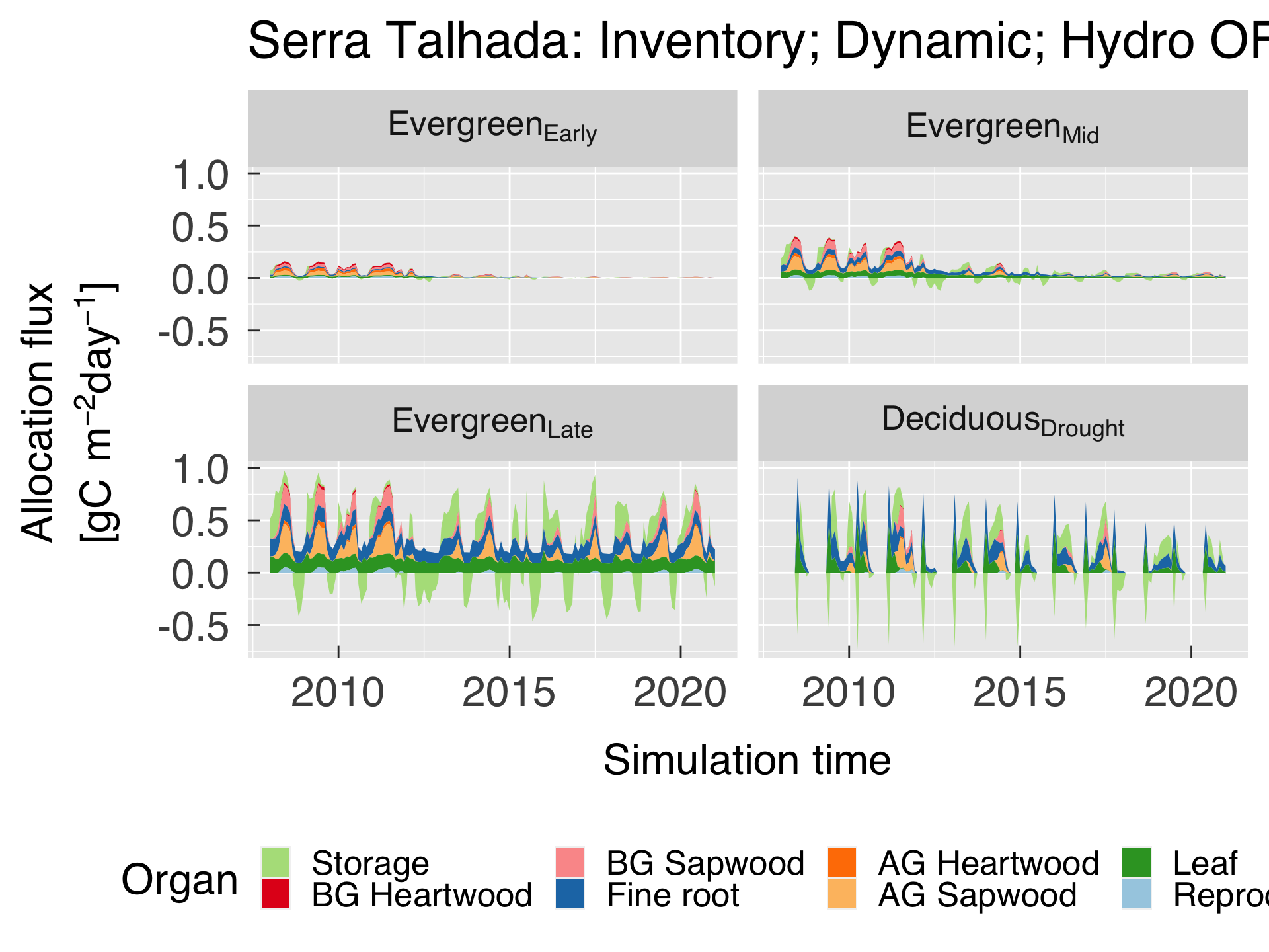
# In case we are to plot NPP by type and size(DBH), reorganise NPP data.
if (plot_alloc_dbh){
   # Re-order NPP so it becomes all in one tibble.
   allocdbh = bydbh %>%
      filter( dbh != 1) %>%
      select_at(all_of(c("time","dbh",allocvar$vnam))) %>%
      pivot_longer(cols=allocvar$vnam,names_to="otype",values_to="npp") %>%
      mutate( otype = factor(allocvar$desc[match(otype,allocvar$vnam)],levels=allocvar$desc    )
            , dbh   = factor(dbhinfo$desc[match(dbh  ,dbhinfo$id  )],levels=dbhinfo$desc[-1]) )

   # Initialise plot (decide whether to plot lines or stacks).
   gg_mdbh = ggplot(data=allocdbh,aes(x=time,y=npp,group=otype,fill=otype))
   gg_mdbh = gg_mdbh + facet_wrap( ~ dbh, ncol = 3L, labeller = label_parsed)
   gg_mdbh = gg_mdbh + scale_fill_manual(name="Organ",labels=allocvar$desc,values=allocvar$colour)
   gg_mdbh = gg_mdbh + geom_area(position=position_stack(reverse = FALSE),show.legend = TRUE)
   gg_mdbh = gg_mdbh + labs(title=case_desc)
   gg_mdbh = gg_mdbh + scale_x_datetime(date_labels=gg_tfmt)
   gg_mdbh = gg_mdbh + xlab("Simulation time")
   gg_mdbh = gg_mdbh + ylab(desc.unit(desc="Allocation flux",unit=untab$gcom2oday,twolines=TRUE))
   gg_mdbh = gg_mdbh + theme_grey( base_size = gg_ptsz, base_family = "Helvetica",base_line_size = 0.5,base_rect_size =0.5)
   gg_mdbh = gg_mdbh + theme( axis.text.x       = element_text( size   = gg_ptsz
                                                              , margin = unit(rep(0.35,times=4),"cm")
                                                              )#end element_text
                            , axis.text.y       = element_text( size   = gg_ptsz
                                                              , margin = unit(rep(0.35,times=4),"cm")
                                                              )#end element_text
                            , plot.title        = element_text( size = gg_ptsz)
                            , axis.ticks.length = unit(-0.25,"cm")
                            , legend.position   = "bottom"
                            , legend.direction  = "horizontal"
                            )#end theme

   # Save plots.
   for (d in sequence(ndevice)){
      m_output = paste0("alloc-bydbh-",case_fpref,".",gg_device[d])
      dummy    = ggsave( filename = m_output
                       , plot     = gg_mdbh
                       , device   = gg_device[d]
                       , path     = tsalloc_path
                       , width    = gg_width*2
                       , height   = gg_height*2
                       , units    = gg_units
                       , dpi      = gg_depth
                       )#end ggsave

   }#end for (d in sequence(ndevice))

   # If sought, plot images on screen
   if (gg_screen) gg_mdbh

}#end if (plot_alloc_dbh)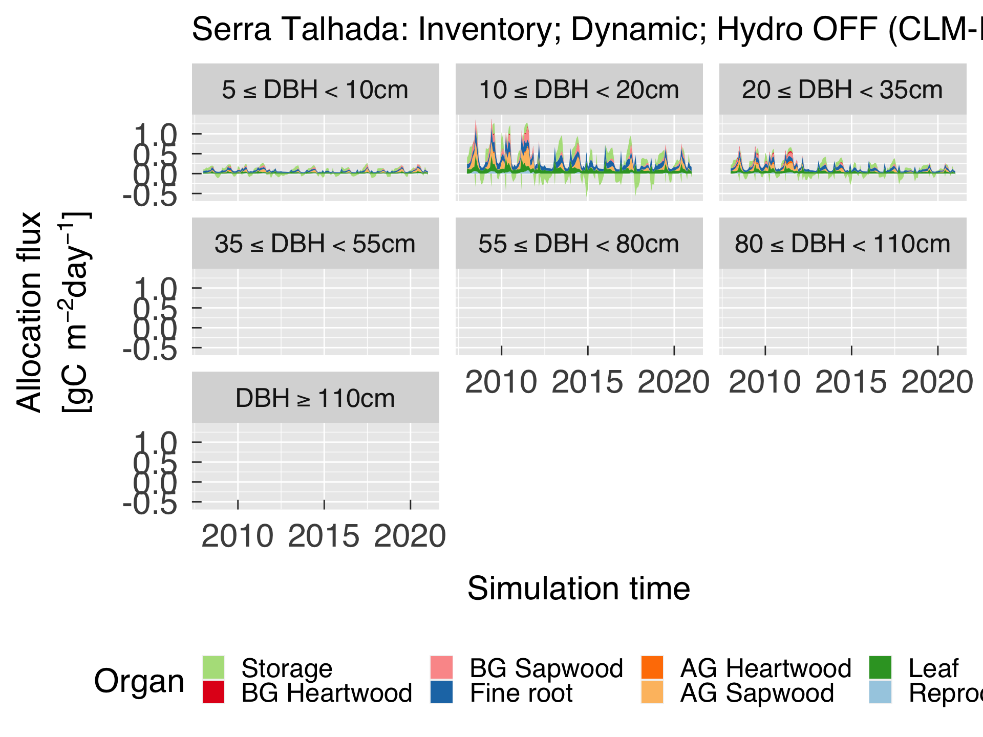
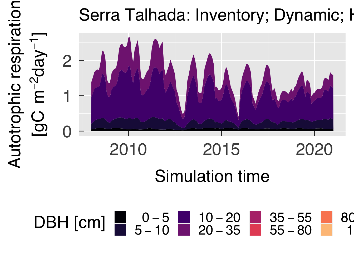
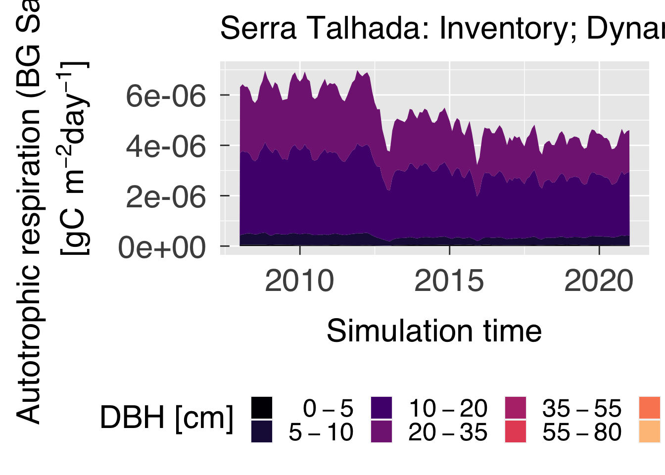
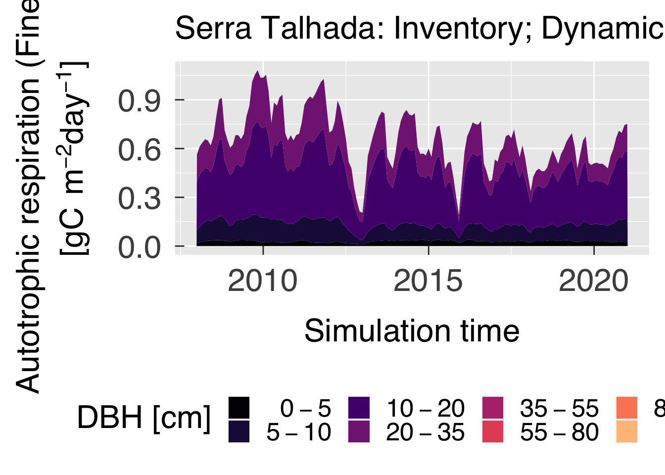
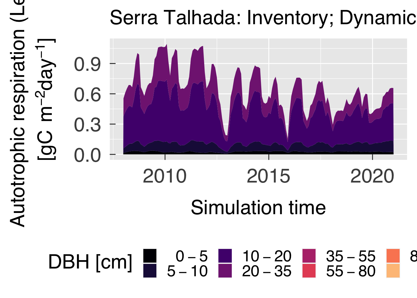
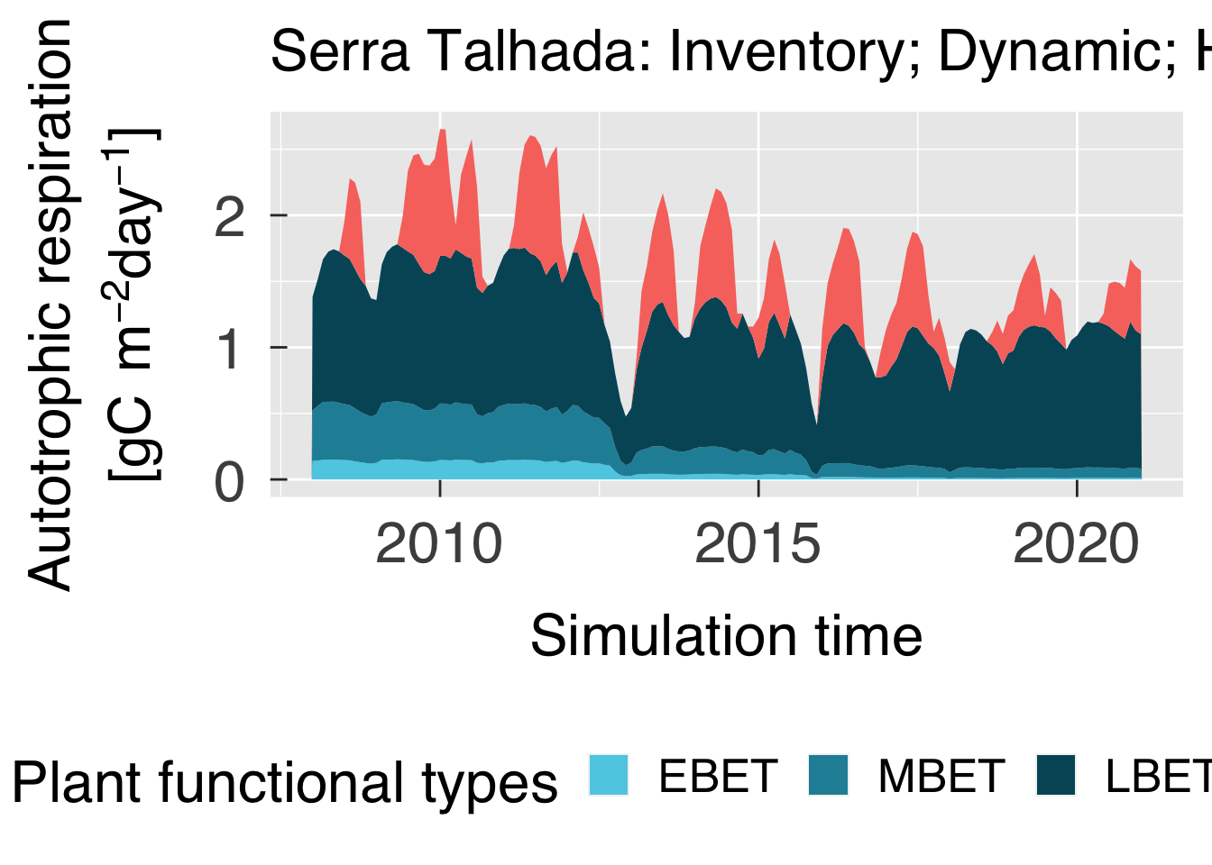
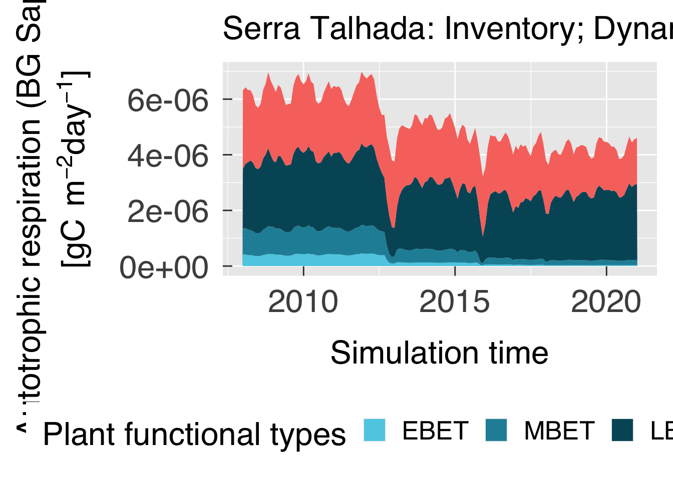
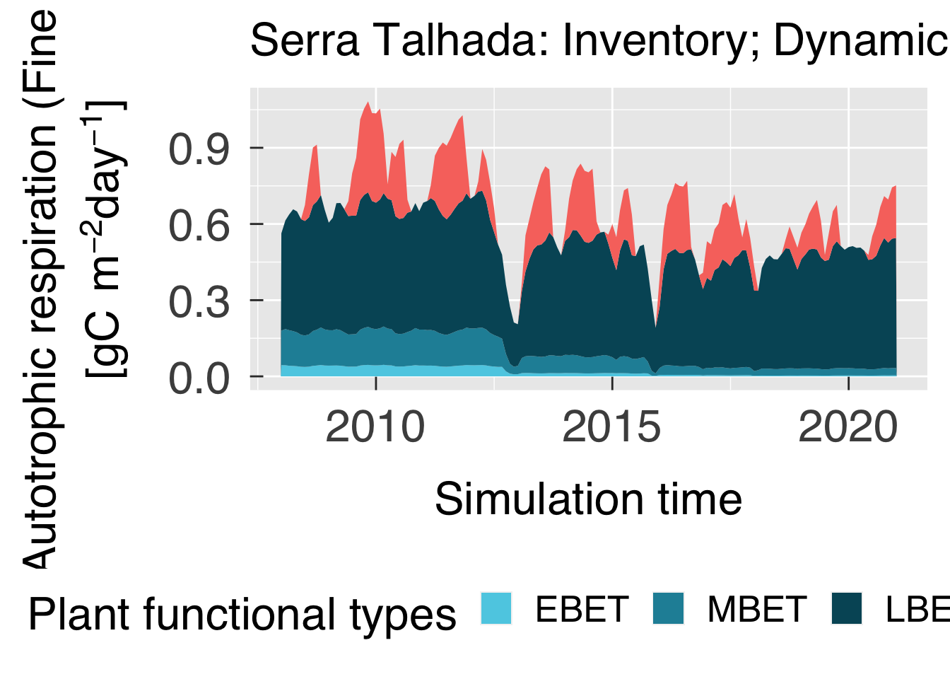
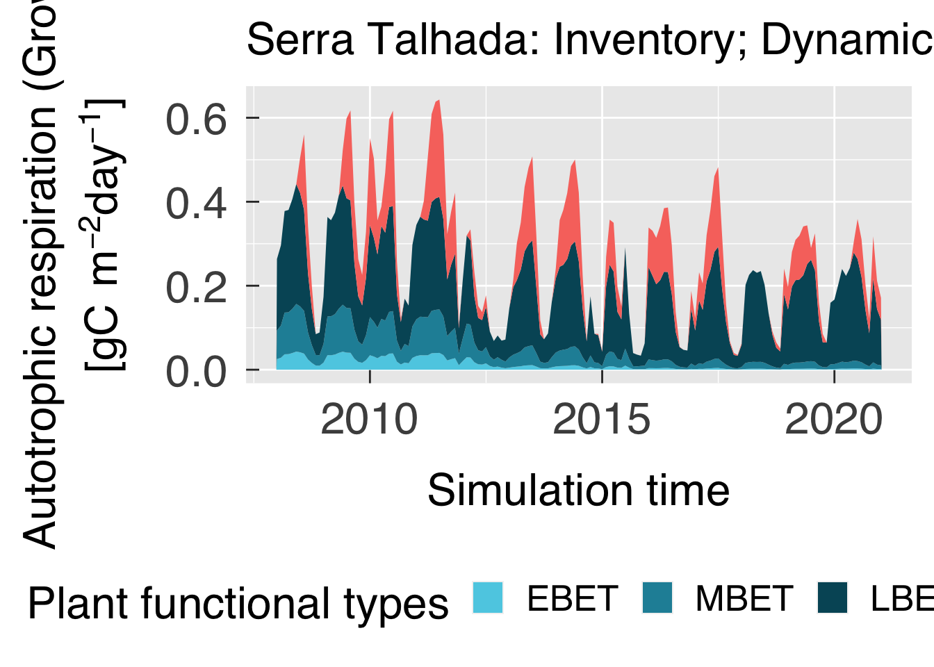
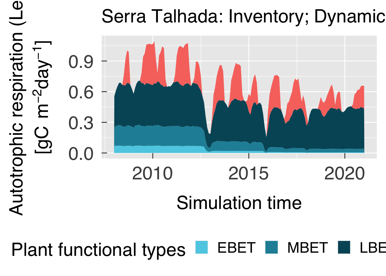
Plot time series of autotrophic respiration by organ type (multiple panels by PFT or by size/DBH class).
# Select mortality type variables, ensure all of them are present.
autovar        = fatesvar[fatesvar$vtype %in% "ar",]
autovar        = autovar[order(autovar$order),,drop=FALSE]
autovar$desc   = gsub(pattern="Autotrophic respiration \\(",replacement="",x=autovar$desc)
autovar$desc   = gsub(pattern="\\)"         ,replacement="",x=autovar$desc)
nautos         = nrow(autovar)
plot_auto_dbh  = all(autovar$vnam %in% names(bydbh))
plot_auto_pft  = all(autovar$vnam %in% names(bypft))

# In case we are to plot NPP by type and PFT, reorganise NPP data.
if (plot_auto_pft){
   # Re-order NPP so it becomes all in one tibble.
   autopft = bypft %>%
             select_at(all_of(c("time","pft",autovar$vnam))) %>%
             pivot_longer(cols=autovar$vnam,names_to="atype",values_to="ar") %>%
             mutate( atype = factor(autovar$desc[match(atype,autovar$vnam)],levels=autovar$desc )
                   , pft   = factor(pftinfo$parse[match(pft,pftinfo$id)]   ,levels=pftinfo$parse) )


   # Initialise plot (decide whether to plot lines or stacks).
   gg_mpft = ggplot(data=autopft,aes(x=time,y=ar,group=atype,fill=atype))
   gg_mpft = gg_mpft + facet_wrap( ~ pft, ncol = 2, labeller = label_parsed)
   gg_mpft = gg_mpft + scale_fill_manual(name="Organ",labels=autovar$desc,values=autovar$colour)
   gg_mpft = gg_mpft + geom_area(position=position_stack(reverse = FALSE),show.legend = TRUE)
   gg_mpft = gg_mpft + labs(title=case_desc)
   gg_mpft = gg_mpft + scale_x_datetime(date_labels=gg_tfmt)
   gg_mpft = gg_mpft + xlab("Simulation time")
   gg_mpft = gg_mpft + ylab(desc.unit(desc="Autotrophic respiration",unit=untab$gcom2oday,twolines=TRUE))
   gg_mpft = gg_mpft + theme_grey( base_size = gg_ptsz, base_family = "Helvetica",base_line_size = 0.5,base_rect_size =0.5)
   gg_mpft = gg_mpft + theme( axis.text.x       = element_text( size   = gg_ptsz
                                                              , margin = unit(rep(0.35,times=4),"cm")
                                                              )#end element_text
                            , axis.text.y       = element_text( size   = gg_ptsz
                                                              , margin = unit(rep(0.35,times=4),"cm")
                                                              )#end element_text
                            , axis.ticks.length = unit(-0.25,"cm")
                            , legend.position   = "bottom"
                            , legend.direction  = "horizontal"
                            )#end theme

   # Save plots.
   for (d in sequence(ndevice)){
      m_output = paste0("ar-bypft-",case_fpref,".",gg_device[d])
      dummy    = ggsave( filename = m_output
                       , plot     = gg_mpft
                       , device   = gg_device[d]
                       , path     = tsauto_path
                       , width    = gg_width
                       , height   = gg_height
                       , units    = gg_units
                       , dpi      = gg_depth
                       )#end ggsave

   }#end for (d in sequence(ndevice))

   # If sought, plot images on screen
   if (gg_screen) gg_mpft

}#end if (plot_auto_pft)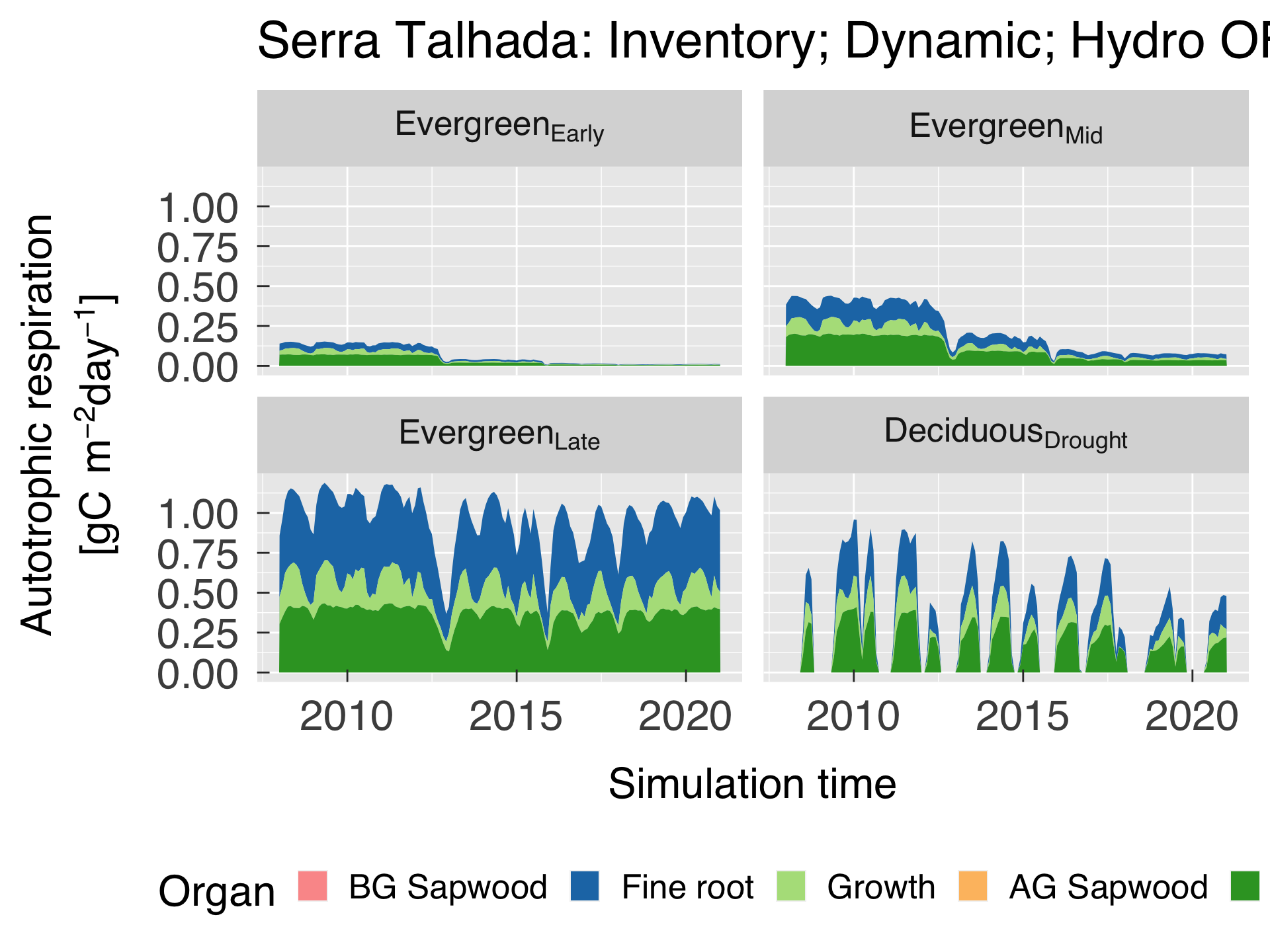
# In case we are to plot NPP by type and size(DBH), reorganise NPP data.
if (plot_auto_dbh){
   # Re-order NPP so it becomes all in one tibble.
   autodbh = bydbh %>%
             filter( dbh != 1) %>%
             select_at(all_of(c("time","dbh",autovar$vnam))) %>%
             pivot_longer(cols=autovar$vnam,names_to="atype",values_to="ar") %>%
             mutate( atype = factor(autovar$desc[match(atype,autovar$vnam)],levels=autovar$desc    )
                   , dbh   = factor(dbhinfo$desc[match(dbh  ,dbhinfo$id  )],levels=dbhinfo$desc[-1]) )

   # Initialise plot (decide whether to plot lines or stacks).
   gg_mdbh = ggplot(data=autodbh,aes(x=time,y=ar,group=atype,fill=atype))
   gg_mdbh = gg_mdbh + facet_wrap( ~ dbh, ncol = 3L, labeller = label_parsed)
   gg_mdbh = gg_mdbh + scale_fill_manual(name="Organ",labels=autovar$desc,values=autovar$colour)
   gg_mdbh = gg_mdbh + geom_area(position=position_stack(reverse = FALSE),show.legend = TRUE)
   gg_mdbh = gg_mdbh + labs(title=case_desc)
   gg_mdbh = gg_mdbh + scale_x_datetime(date_labels=gg_tfmt)
   gg_mdbh = gg_mdbh + xlab("Simulation time")
   gg_mdbh = gg_mdbh + ylab(desc.unit(desc="Autotrophic Respiration",unit=untab$gcom2oday,twolines=TRUE))
   gg_mdbh = gg_mdbh + theme_grey( base_size = gg_ptsz, base_family = "Helvetica",base_line_size = 0.5,base_rect_size =0.5)
   gg_mdbh = gg_mdbh + theme( axis.text.x       = element_text( size   = gg_ptsz
                                                              , margin = unit(rep(0.35,times=4),"cm")
                                                              )#end element_text
                            , axis.text.y       = element_text( size   = gg_ptsz
                                                              , margin = unit(rep(0.35,times=4),"cm")
                                                              )#end element_text
                            , plot.title        = element_text( size = gg_ptsz)
                            , axis.ticks.length = unit(-0.25,"cm")
                            , legend.position   = "bottom"
                            , legend.direction  = "horizontal"
                            )#end theme

   # Save plots.
   for (d in sequence(ndevice)){
      m_output = paste0("ar-bydbh-",case_fpref,".",gg_device[d])
      dummy    = ggsave( filename = m_output
                       , plot     = gg_mdbh
                       , device   = gg_device[d]
                       , path     = tsauto_path
                       , width    = gg_width*2
                       , height   = gg_height*2
                       , units    = gg_units
                       , dpi      = gg_depth
                       )#end ggsave

   }#end for (d in sequence(ndevice))

   # If sought, plot images on screen
   if (gg_screen) gg_mdbh

}#end if (plot_auto_dbh)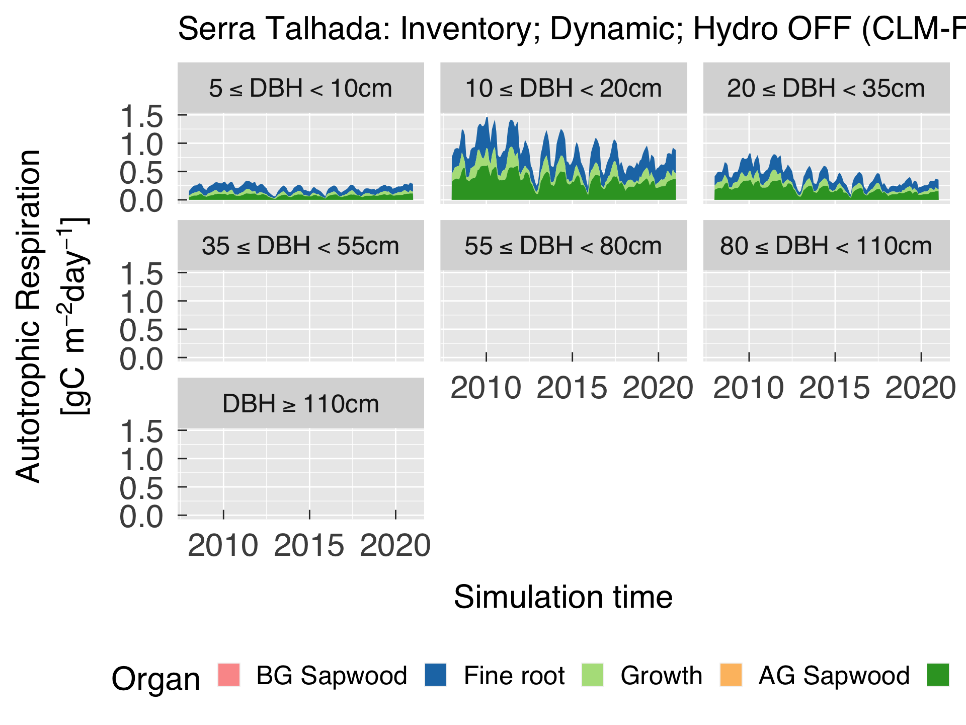
Plot time series of drought-deciduous phenology variables (status). These are very specific plots, so we do not try to automate them.
# Select mortality type variables, ensure all of them are present.
plot_dphen     = all(dphenvar$vnam %in% names(dphen))


# In case we are to plot drought-deciduous plots, reorganise data.
if (plot_dphen){

   # Reorganise phenology data
   dshow = dphen %>%
           mutate( tmin       = time
                 , tmax       = time + make_difftime(day=days_in_month(time))
                 , dstatus    = as.integer(round(dstatus))
                 , mean_smp   = ifelse(test = mean_swc == 0., yes=NA_real_,no=mean_smp)
                 , mean_swc   = ifelse(test = mean_swc == 0., yes=NA_real_,no=mean_swc)
                 , ndays      = ifelse ( test=dstatus %in% c(2,3), yes=ndays_on , no = ndays_off)
                 , ddesc      = factor(x=dstatus,levels=dphinfo$id ) )

   # Match colours and legend for soil moisture
   mst         = match(x=c("mean_swc","mean_smp"),table=dphenvar$vnam)
   mst_names   = dphenvar$vnam  [mst]
   mst_labels  = dphenvar$desc  [mst]
   mst_colours = dphenvar$colour[mst]
   mst_units   = dphenvar$unit  [mst]


   # Loop through PFTs to plot
   pft_loop = which(pftinfo$drdecid)
   gg_mpft  = list()
   for (p in pft_loop){
      # Select PFT
      p_id      = pftinfo$id  [p]
      p_key     = pftinfo$key [p]
      p_desc    = pftinfo$desc[p]
      p_mthresh = pftinfo$mthresh[p]
      p_dthresh = pftinfo$dthresh[p]
      p_show = dshow %>% filter( pft == p_id)

      # Find range for the soil water content
      if (! ( (p_mthresh*p_dthresh) %ge% 0.) ){
         cat0(" Current settings for PFT ",p_id, "(",p_desc,").")
         cat0(" mthresh = ",p_mthresh)
         cat0(" dthresh = ",p_dthresh)
         stop(" Invalid settings for moisture thresholds. Both must be either negative or positive! ")
      }else if( ! (p_mthresh %gt% p_dthresh)){
         cat0(" Current settings for PFT ",p_id, "(",p_desc,").")
         cat0(" mthresh = ",p_mthresh)
         cat0(" dthresh = ",p_dthresh)
         stop(" Invalid settings for moisture thresholds. Variable \"mthresh\" must be greater than \"dthresh\"! ")
      }else if( p_dthresh %ge% 0.){
         swc_lwr   = min(c(p_dthresh,p_show$mean_swc),na.rm=TRUE)
         swc_upr   = max(c(p_mthresh,p_show$mean_swc),na.rm=TRUE)
         swc_lwr   = swc_lwr - 0.05 * (swc_upr - swc_lwr)
         smp_lwr   = min(p_show$mean_smp,na.rm=TRUE)
         smp_upr   = max(p_show$mean_smp,na.rm=TRUE)
         lnsmp_lwr = -log(-smp_lwr)
         lnsmp_upr = -log(-smp_upr)
      }else{
         swc_lwr   = min(p_show$mean_swc,na.rm=TRUE)
         swc_upr   = max(p_show$mean_swc,na.rm=TRUE)
         swc_lwr   = swc_lwr - 0.05 * (swc_upr - swc_lwr)
         smp_lwr   = min(c(p_dthresh,p_show$mean_smp),na.rm=TRUE)
         smp_upr   = max(c(p_mthresh,p_show$mean_smp),na.rm=TRUE)
         lnsmp_lwr = -log(-smp_lwr)
         lnsmp_upr = -log(-smp_upr)
      }#end if (! ( (p_mthresh*p_dtrhesh) %ge% 0.) )

      # Create reprojected soil matric potential in the same scale as soil moisture
      v_show = p_show %>%
               mutate( orig_smp = mean_smp
                     , norm_smp = (-log(-orig_smp) - lnsmp_lwr) / (lnsmp_upr - lnsmp_lwr)
                     , mean_smp = swc_lwr + norm_smp * (swc_upr - swc_lwr) ) %>%
               pivot_longer(cols=c("mean_swc","mean_smp"),names_to="mtype",values_to="mvalue")          %>%
               mutate( mtype = factor(dphenvar$desc[match(mtype,dphenvar$vnam)],levels=dphenvar$desc ) )

      # Find breaks for soil water content and soil matric potential
      swc_breaks = identity_trans()$breaks(x=c(swc_lwr,swc_upr))
      swc_labels = sprintf("%g",swc_breaks)
      swc_annot  = desc.unit(desc=NULL,unit=untab[[mst_units[1]]])
      smp_actual = neglog10_trans()$breaks(x=c(smp_lwr,smp_upr))
      smp_breaks = swc_lwr + ( -log(-smp_actual) - lnsmp_lwr) * (swc_upr - swc_lwr) / (lnsmp_upr - lnsmp_lwr)
      # Restrict smp_breaks to the range of soil water content
      smp_keep   = smp_breaks %wr% c(swc_lwr,swc_upr)
      smp_actual = smp_actual[smp_keep]
      smp_labels = sprintf("%g",smp_actual)
      smp_breaks = smp_breaks[smp_keep]
      smp_annot  = desc.unit(desc=NULL,unit=untab[[mst_units[2]]])

      # Find band for the drought phenology
      if (p_dthresh >= 0.0){
         p_show = p_show %>% mutate( stt_lwr = p_dthresh, stt_upr = p_mthresh )
      }else{
         p_show = p_show %>%
                  mutate( stt_lwr = swc_lwr + ( -log(-p_dthresh) - lnsmp_lwr) * (swc_upr - swc_lwr) / (lnsmp_upr - lnsmp_lwr)
                        , stt_upr = swc_lwr + ( -log(-p_mthresh) - lnsmp_lwr) * (swc_upr - swc_lwr) / (lnsmp_upr - lnsmp_lwr) )
      }#end if (p_dthresh >= 0.0)

      # Plot time and phenology status.
      gg_now = ggplot(colour="transparent",fill="transparent")
      gg_now = gg_now  + geom_rect( data        = p_show
                                  , mapping     = aes(xmin=tmin,xmax=tmax,ymin=stt_lwr,ymax=stt_upr,fill=ddesc)
                                  , linetype    = "blank"
                                  , show.legend = TRUE
                                  , inherit.aes = FALSE
                                  )#end geom_rect
      gg_now = gg_now  + scale_fill_manual(name="Status",breaks=as.character(dphinfo$id),labels=dphinfo$desc,values=dphinfo$colour)
      gg_now = gg_now  + geom_line( data        = v_show
                                  , mapping     = aes(x=time,y=mvalue,colour=mtype)
                                  , lwd         = 1.0
                                  , show.legend = TRUE
                                  , inherit.aes = FALSE
                                  )#end geom_line
      gg_now = gg_now  + scale_colour_manual(name="Moisture",labels=mst_labels,values=mst_colours)
      gg_now = gg_now  + guides( fill   = guide_legend(override.aes = list(colour= "transparent"))
                               , colour = guide_legend(override.aes = list(fill  = "transparent"))
                               )#end guides
      gg_now = gg_now  + labs(title=paste0(case_desc," - ",p_desc))
      gg_now = gg_now  + scale_x_datetime(date_labels=gg_tfmt)
      gg_now = gg_now  + scale_y_continuous( name     = swc_annot
                                           , breaks   = swc_breaks
                                           , labels   = swc_labels
                                           , limits   = c(swc_lwr,swc_upr)
                                           , sec.axis = dup_axis( name   = smp_annot
                                                                , breaks = smp_breaks
                                                                , labels = smp_labels
                                                                )#end dup_axis
                                           )#end scale_y_continuous
      gg_now = gg_now  + xlab("Simulation time")
      gg_now = gg_now + theme_grey( base_size = gg_ptsz, base_family = "Helvetica",base_line_size = 0.5,base_rect_size =0.5)
      gg_now = gg_now + theme( axis.text.x       = element_text( size   = gg_ptsz
                                                               , margin = unit(rep(0.35,times=4),"cm")
                                                               )#end element_text
                             , axis.text.y       = element_text( size   = gg_ptsz
                                                               , margin = unit(rep(0.35,times=4),"cm")
                                                               )#end element_text
                             , axis.ticks.length = unit(-0.25,"cm")
                             , legend.position   = "right"
                             , legend.direction  = "vertical"
                             )#end theme

      # Save plots.
      for (d in sequence(ndevice)){
         p_output = paste0("phen-",p_key,"-",case_fpref,".",gg_device[d])
         dummy    = ggsave( filename = p_output
                          , plot     = gg_now
                          , device   = gg_device[d]
                          , path     = tsdphen_path
                          , width    = gg_width
                          , height   = gg_height
                          , units    = gg_units
                          , dpi      = gg_depth
                          )#end ggsave

      }#end for (d in sequence(ndevice))

      # Append plot to list
      gg_mpft[[p_key]] = gg_now
   }#end for (p in pft_loop)

   # If sought, plot images on screen
   if (gg_screen) gg_mpft
}#end if (plot_auto_pft)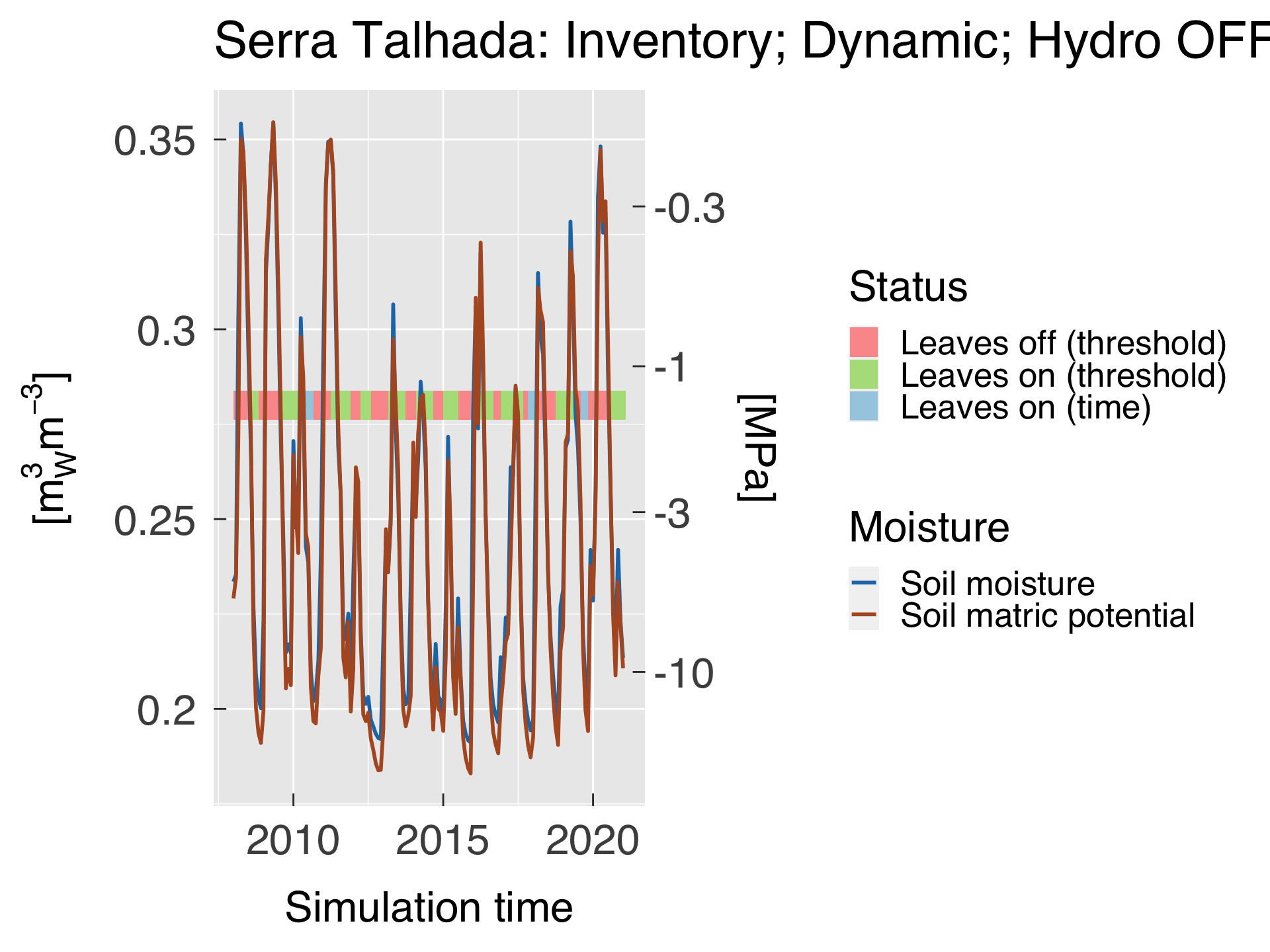
Plot time series of drought-deciduous phenology variables (elongation factor). These are very specific plots, so we do not try to automate them.
# Select mortality type variables, ensure all of them are present.
plot_dphen     = all(dphenvar$vnam %in% names(dphen))


# In case we are to plot drought-deciduous plots, reorganise data.
if (plot_dphen){

   # Reorganise phenology data
   dshow = dphen %>%
           mutate( tmin       = time
                 , tmax       = time + make_difftime(day=days_in_month(time))
                 , mean_smp   = ifelse(test = mean_swc == 0., yes=NA_real_,no=mean_smp)
                 , mean_swc   = ifelse(test = mean_swc == 0., yes=NA_real_,no=mean_swc)
                 , ndays      = ifelse ( test=dstatus %in% c(2,3), yes=ndays_on , no = ndays_off)
                 , ddesc      = factor(x=dstatus,levels=dphinfo$id ) )

   # Match colours and legend for soil moisture
   mst         = match(x=c("mean_swc","mean_smp"),table=dphenvar$vnam)
   mst_names   = dphenvar$vnam  [mst]
   mst_labels  = dphenvar$desc  [mst]
   mst_colours = dphenvar$colour[mst]
   mst_units   = dphenvar$unit  [mst]


   # Loop through PFTs to plot
   pft_loop = which(pftinfo$drdecid)
   gg_mpft  = list()
   for (p in pft_loop){
      # Select PFT
      p_id      = pftinfo$id  [p]
      p_key     = pftinfo$key [p]
      p_desc    = pftinfo$desc[p]
      p_mthresh = pftinfo$mthresh[p]
      p_dthresh = pftinfo$dthresh[p]
      p_show = dshow %>% filter( pft == p_id)

      # Find range for the soil water content
      if (! ( (p_mthresh*p_dthresh) %ge% 0.) ){
         cat0(" Current settings for PFT ",p_id, "(",p_desc,").")
         cat0(" mthresh = ",p_mthresh)
         cat0(" dthresh = ",p_dthresh)
         stop(" Invalid settings for moisture thresholds. Both must be either negative or positive! ")
      }else if( ! (p_mthresh %gt% p_dthresh)){
         cat0(" Current settings for PFT ",p_id, "(",p_desc,").")
         cat0(" mthresh = ",p_mthresh)
         cat0(" dthresh = ",p_dthresh)
         stop(" Invalid settings for moisture thresholds. Variable \"mthresh\" must be greater than \"dthresh\"! ")
      }else if( p_dthresh %ge% 0.){
         swc_lwr   = min(c(p_dthresh,p_show$mean_swc),na.rm=TRUE)
         swc_upr   = max(c(p_mthresh,p_show$mean_swc),na.rm=TRUE)
         swc_lwr   = swc_lwr - 0.05 * (swc_upr - swc_lwr)
         smp_lwr   = min(p_show$mean_smp,na.rm=TRUE)
         smp_upr   = max(p_show$mean_smp,na.rm=TRUE)
         lnsmp_lwr = -log(-smp_lwr)
         lnsmp_upr = -log(-smp_upr)
      }else{
         swc_lwr   = min(p_show$mean_swc,na.rm=TRUE)
         swc_upr   = max(p_show$mean_swc,na.rm=TRUE)
         swc_lwr   = swc_lwr - 0.05 * (swc_upr - swc_lwr)
         smp_lwr   = min(c(p_dthresh,p_show$mean_smp),na.rm=TRUE)
         smp_upr   = max(c(p_mthresh,p_show$mean_smp),na.rm=TRUE)
         lnsmp_lwr = -log(-smp_lwr)
         lnsmp_upr = -log(-smp_upr)
      }#end if (! ( (p_mthresh*p_dtrhesh) %ge% 0.) )

      # Create reprojected soil matric potential in the same scale as soil moisture
      v_show = p_show %>%
               mutate( orig_smp = mean_smp
                     , norm_smp = (-log(-orig_smp) - lnsmp_lwr) / (lnsmp_upr - lnsmp_lwr)
                     , mean_smp = swc_lwr + norm_smp * (swc_upr - swc_lwr) ) %>%
               pivot_longer(cols=c("mean_swc","mean_smp"),names_to="mtype",values_to="mvalue")          %>%
               mutate( mtype = factor(dphenvar$desc[match(mtype,dphenvar$vnam)],levels=dphenvar$desc ) )

      # Find breaks for soil water content and soil matric potential
      swc_breaks = identity_trans()$breaks(x=c(swc_lwr,swc_upr))
      swc_labels = sprintf("%g",swc_breaks)
      swc_annot  = desc.unit(desc=NULL,unit=untab[[mst_units[1]]])
      smp_actual = neglog10_trans()$breaks(x=c(smp_lwr,smp_upr))
      smp_breaks = swc_lwr + ( -log(-smp_actual) - lnsmp_lwr) * (swc_upr - swc_lwr) / (lnsmp_upr - lnsmp_lwr)
      # Restrict smp_breaks to the range of soil water content
      smp_keep   = smp_breaks %wr% c(swc_lwr,swc_upr)
      smp_actual = smp_actual[smp_keep]
      smp_labels = sprintf("%g",smp_actual)
      smp_breaks = smp_breaks[smp_keep]
      smp_annot  = desc.unit(desc=NULL,unit=untab[[mst_units[2]]])

      # Find band for the drought phenology
      if (p_dthresh >= 0.0){
         p_show = p_show %>% mutate( stt_lwr = p_dthresh, stt_upr = p_mthresh )
      }else{
         p_show = p_show %>%
                  mutate( stt_lwr = swc_lwr + ( -log(-p_dthresh) - lnsmp_lwr) * (swc_upr - swc_lwr) / (lnsmp_upr - lnsmp_lwr)
                        , stt_upr = swc_lwr + ( -log(-p_mthresh) - lnsmp_lwr) * (swc_upr - swc_lwr) / (lnsmp_upr - lnsmp_lwr) )
      }#end if (p_dthresh >= 0.0)

      # Create colours palette
      e_colours = rev(viridis::plasma(n=5))
      e_palette = grDevices::colorRampPalette(colors=e_colours,space="Lab")

      # Plot time and phenology status.
      gg_now = ggplot(colour="transparent",fill="transparent")
      gg_now = gg_now  + geom_rect( data        = p_show
                                  , mapping     = aes(xmin=tmin,xmax=tmax,ymin=stt_lwr,ymax=stt_upr,fill=elong_factor)
                                  , linetype    = "blank"
                                  , show.legend = TRUE
                                  , inherit.aes = FALSE
                                  )#end geom_rect
      gg_now = gg_now  + scale_fill_gradientn( name    = "Elongation"
                                             , colours = e_palette(n=gg_ncolours)
                                             , limits  = c(0,1)
                                             , labels  = label_number()
                                             )#end scale_fill_gradientn
      gg_now = gg_now  + geom_line( data        = v_show
                                  , mapping     = aes(x=time,y=mvalue,colour=mtype)
                                  , lwd         = 1.0
                                  , show.legend = TRUE
                                  , inherit.aes = FALSE
                                  )#end geom_line
      gg_now = gg_now  + scale_colour_manual(name="Moisture",labels=mst_labels,values=mst_colours)
      gg_now = gg_now  + guides( colour = guide_legend(override.aes = list(fill  = "transparent")) )
      gg_now = gg_now  + labs(title=paste0(case_desc," - ",p_desc))
      gg_now = gg_now  + scale_x_datetime(date_labels=gg_tfmt)
      gg_now = gg_now  + scale_y_continuous( name     = swc_annot
                                           , breaks   = swc_breaks
                                           , labels   = swc_labels
                                           , limits   = c(swc_lwr,swc_upr)
                                           , sec.axis = dup_axis( name   = smp_annot
                                                                , breaks = smp_breaks
                                                                , labels = smp_labels
                                                                )#end dup_axis
                                           )#end scale_y_continuous
      gg_now = gg_now  + xlab("Simulation time")
      gg_now = gg_now + theme_grey( base_size = gg_ptsz, base_family = "Helvetica",base_line_size = 0.5,base_rect_size =0.5)
      gg_now = gg_now + theme( axis.text.x       = element_text( size   = gg_ptsz
                                                               , margin = unit(rep(0.35,times=4),"cm")
                                                               )#end element_text
                             , axis.text.y       = element_text( size   = gg_ptsz
                                                               , margin = unit(rep(0.35,times=4),"cm")
                                                               )#end element_text
                             , axis.ticks.length = unit(-0.25,"cm")
                             , legend.position   = "right"
                             , legend.direction  = "vertical"
                             )#end theme

      # Save plots.
      for (d in sequence(ndevice)){
         p_output = paste0("elongf-",p_key,"-",case_fpref,".",gg_device[d])
         dummy    = ggsave( filename = p_output
                          , plot     = gg_now
                          , device   = gg_device[d]
                          , path     = tsdphen_path
                          , width    = gg_width
                          , height   = gg_height
                          , units    = gg_units
                          , dpi      = gg_depth
                          )#end ggsave

      }#end for (d in sequence(ndevice))

      # Append plot to list
      gg_mpft[[p_key]] = gg_now
   }#end for (p in pft_loop)

   # If sought, plot images on screen
   if (gg_screen) gg_mpft
}#end if (plot_auto_pft)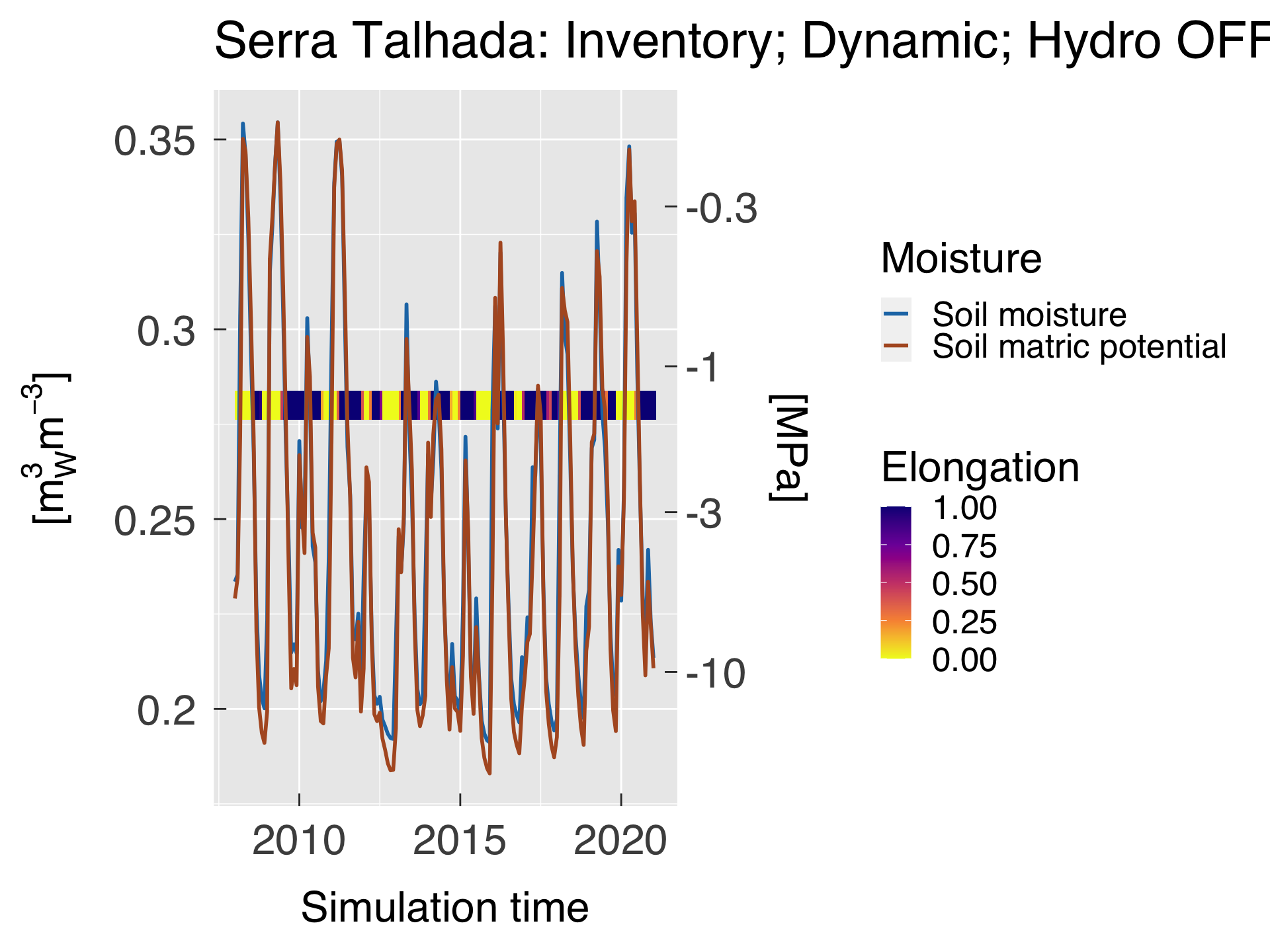
Plot the time series of soil data:
cat0(" + Plot time series of soil variables.")

# Define the deepest layer to show.
slz_show = max(slz_deepest,slzinfo$slz[n_bedrock])

# Modify data for plotting, but keep the input unchanged
h_soi2d  = soi2d %>%
           filter ( slzinfo$show[slz]) %>%
           mutate( tmin = time
                 , tmax = time + make_difftime(day=days_in_month(time))
                 , zmin = slzinfo$slz_lwr[slz]
                 , zmax = slzinfo$slz_upr[slz]
                 , slz  = slzinfo$slz    [slz]
                 )#end mutate

# Define limits for the soil plot
slz_limit = range(c(h_soi2d$zmin,h_soi2d$zmax))

# Select variables to plot
soi_loop = which(hlm2dsoi$vnam %in% names(soi2d))

gg_soil   = list()
for (h in soi_loop){
   # Match variables.
   h_vnam   = hlm2dsoi$vnam  [h]
   h_desc   = hlm2dsoi$desc  [h]
   h_short  = hlm2dsoi$short [h]
   h_unit   = hlm2dsoi$unit  [h]
   h_csch   = gsub (pattern="^i_" ,replacement="",x=hlm2dsoi$csch[h])
   h_cinv   = grepl(pattern="^i_"                ,x=hlm2dsoi$csch[h])
   h_mirror = hlm2dsoi$mirror[h]
   h_trans  = hlm2dsoi$trans [h]
   cat0("   - ",h_desc,".")


   # If this is a log-transformed or sqrt-transformed data, eliminate negative values (and zeroes for log)
   if (grepl(pattern="^log",x=h_trans)){
      h_soi2d[[h_vnam]] = ifelse( test = h_soi2d[[h_vnam]] %gt% 0., yes=h_soi2d[[h_vnam]], no = NA_real_)
   }else if (grepl(pattern="^sqrt",x=h_trans)){
      h_soi2d[[h_vnam]] = ifelse( test = h_soi2d[[h_vnam]] %ge% 0., yes=h_soi2d[[h_vnam]], no = NA_real_)
   }#end if (grepl(pattern="^log",x=h_trans))

   # Plot figure only if there is anything to show.
   if (any(is.finite(h_soi2d[[h_vnam]]))){


      # Find bounds for plot
      h_bounds = find_bounds(x=h_soi2d[[h_vnam]],ci_level=ci_level,mirror=h_mirror,trans=paste0(h_trans,"_trans"))
      h_lwr    = h_bounds[1]
      h_upr    = h_bounds[2]
      h_soi2d  = h_soi2d %>% mutate( across(all_of(h_vnam), ~ bounded(.x,x_lwr=h_lwr,x_upr=h_upr)))

      # Find colours and levels
      if (h_csch %in% brewer_pal_info){
         h_colours = RColorBrewer::brewer.pal(n=5,name=h_csch)
      }else if (h_csch %in% viridis_pal_info){
         h_colours = viridis::viridis(n=5,option=h_csch)
      }else{
         h_csch    = match.fun(h_csch)
         h_colours = h_csch(n=5)
      }#end if (v_cnorm %in% brewer_pal_info)

      # Invert colours if we should use reverse
      if(h_cinv) h_colours = rev(h_colours)

      # Create colour palette
      h_palette = grDevices::colorRampPalette(colors=h_colours,space="Lab")

      # Make key title
      h_keytitle = desc.unit( desc = h_short, unit = untab[[h_unit]], dxpr = TRUE)

      # Initialise 2-D plot.
      gg_now = ggplot( data    = h_soi2d
                     , mapping = aes_string( x    = "time"
                                           , y    = "slz"
                                           , xmin = "tmin"
                                           , xmax = "tmax"
                                           , ymin = "zmin"
                                           , ymax = "zmax"
                                           , fill = h_vnam
                                           )#end aes_string
                     )#end ggplot
      gg_now = gg_now + geom_rect( na.rm = TRUE, show.legend = TRUE)
      gg_now = gg_now + scale_x_datetime(date_labels=gg_tfmt)
      gg_now = gg_now + scale_y_continuous(limits=slz_limit,trans="neglog10",labels=label_number())
      gg_now = gg_now + scale_fill_gradientn(colours=h_palette(n=gg_ncolours),trans=h_trans,limits=h_bounds,labels=label_number())
      gg_now = gg_now + labs(title=case_desc)
      gg_now = gg_now + xlab("Simulation time")
      gg_now = gg_now + ylab(desc.unit(desc="Soil depth",unit=untab$m))
      gg_now = gg_now + labs(fill = h_keytitle)
      gg_now = gg_now + theme_grey( base_size      = gg_ptsz
                                  , base_family    = "Helvetica"
                                  , base_line_size = 0.5
                                  , base_rect_size = 0.5
                                  )#end theme_grey
      gg_now = gg_now + theme( axis.text.x       = element_text( size   = gg_ptsz
                                                               , margin = unit(rep(0.35,times=4),"cm")
                                                               )#end element_text
                             , axis.text.y       = element_text( size   = gg_ptsz
                                                               , margin = unit(rep(0.35,times=4),"cm")
                                                               )#end element_text
                             , plot.title        = element_text( size = gg_ptsz)
                             , axis.ticks.length = unit(-0.25,"cm")
                             , legend.title      = element_text( size = gg_ptsz * 0.6)
                             , legend.position   = "right"
                             , legend.direction  = "vertical"
                             , plot.margin       = unit(c(0,0,0,0), "mm")
                             )#end theme

     # Save plot in every format requested.
     for (d in sequence(ndevice)){
        h_output = paste0(h_vnam,"-tssoil-",case_fpref,".",gg_device[d])
        dummy = ggsave( filename = h_output
                      , plot     = gg_now
                      , device   = gg_device[d]
                      , path     = tssoil_path
                      , width    = gg_width
                      , height   = gg_height
                      , units    = gg_units
                      , dpi      = gg_depth
                      )#end ggsave
      }#end for (o in sequence(nout))

      # Write plot settings to the list.
      gg_soil[[h_vnam]] = gg_now

   }#end if (any(is.finite(h_soi2d[[h_vnam]])))

}#end for (h in sequence(nhlm2dsoi))


# If sought, plot images on screen
if (gg_screen) gg_soil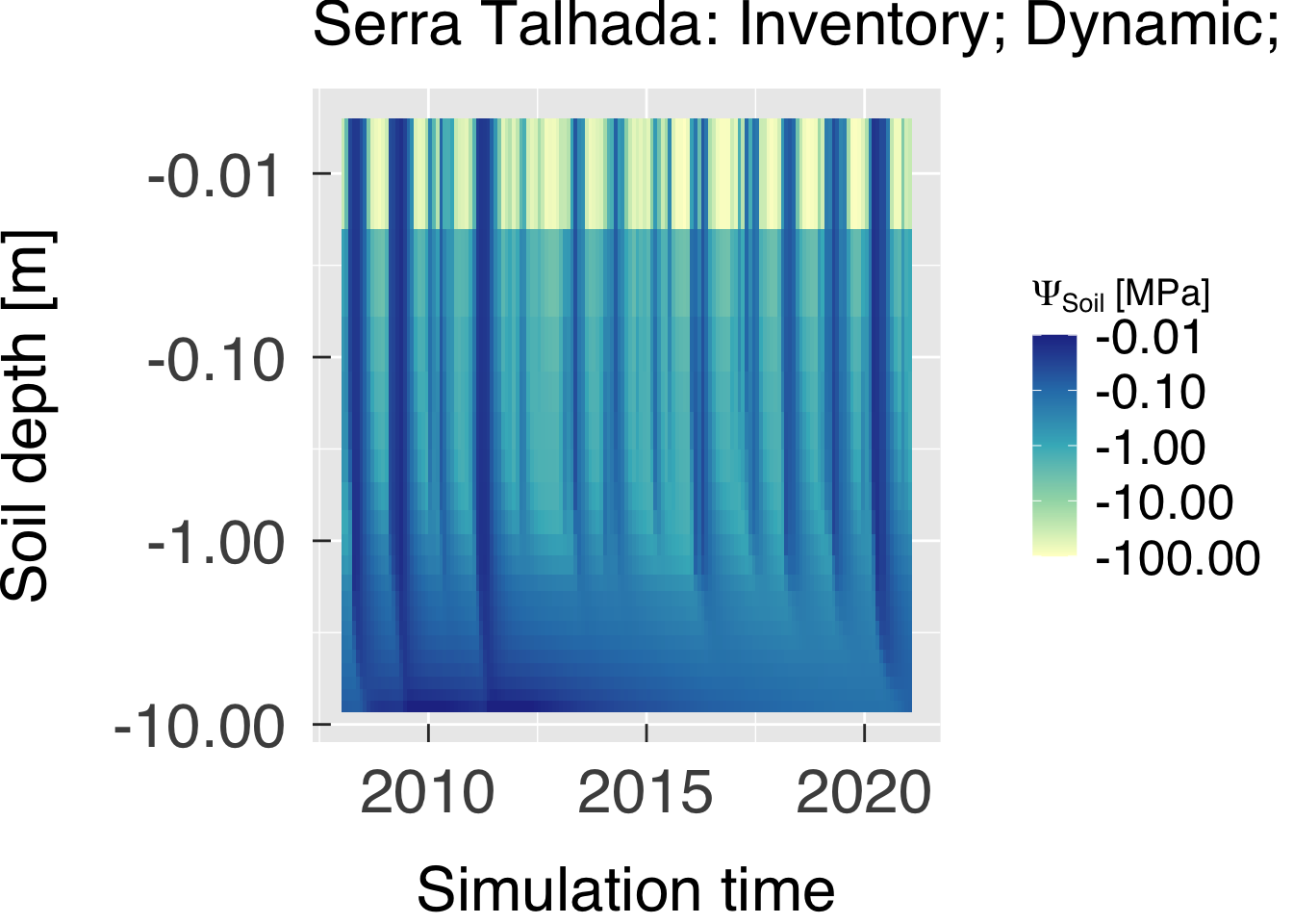
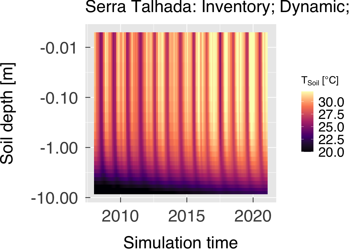
Plot the time series by size and PFT class as heat maps:
cat0(" + Plot heat maps of variables by time, size class, and PFT.")


# Modify data for plotting, but keep the input unchanged
f_bydap  = bydap %>%
           mutate( tmin = time
                 , tmax = time + make_difftime(day=days_in_month(time))
                 , dmin = dbhinfo$dbh_lwr[dbh]
                 , dmax = dbhinfo$dbh_upr[dbh]
                 , dmax = ifelse( is.finite(dmax),dmax,dbhinfo$dbh[ndbhs]+10)
                 , dbh  = dbhinfo$dbh    [dbh]
                 , pft  = factor(x=pftinfo$short[match(pft,pftinfo$id)],levels=pftinfo$short)
                 )#end mutate

# Define limits for the soil plot
dbh_limit = range(c(f_bydap$dmin,f_bydap$dmax))


# Select variables to plot
dap_loop = which(fatesvar$vnam %in% names(bydap))

# Remove data from empty classes
zero_und = f_bydap$fates_nplant_ustory %eq% 0.
zero_can = f_bydap$fates_nplant_canopy %eq% 0.
zero_tot = f_bydap$fates_nplant        %eq% 0.


gg_dap   = list()

for (f in dap_loop){
   # Match variables.
   f_vnam   = fatesvar$vnam     [f]
   f_unit   = fatesvar$dp_unit  [f]
   f_desc   = fatesvar$desc     [f]
   f_indvar = fatesvar$dp_indvar[f]
   f_dbh01  = fatesvar$dbh01    [f]
   f_mirror = fatesvar$mirror   [f]
   f_trans  = fatesvar$trans    [f]

   # Find variables that need some transformations
   f_vund   = grepl(pattern="ustory",x=f_vnam)
   f_vcan   = grepl(pattern="canopy",x=f_vnam)
   f_mult   = eval(parse(text=fatesvar$mult_dp[f]))
   f_cschm  = gsub (pattern="^i_" ,replacement="",x=fatesvar$cschm [f])
   f_csinv  = grepl(pattern="^i_"                ,x=fatesvar$cschm [f])
   f_trfun  = paste0(fatesvar$trans[f],"_trans")

   cat0("   - ",f_desc,".")

   # Eliminate data from clases with zero population. We must check for understory and canopy classes too.
   if (f_indvar %in% "ustory"){
      # Scale by understory population
      f_bydap[[f_vnam]] = ifelse( test = zero_und, yes = NA_real_, no = f_bydap[[f_vnam]]/f_bydap$fates_nplant_ustory)
   }else if (f_indvar %in% "canopy"){
      # Scale by canopy population
      f_bydap[[f_vnam]] = ifelse( test = zero_can, yes = NA_real_, no = f_bydap[[f_vnam]]/f_bydap$fates_nplant_canopy)
   }else if (f_indvar %in% "total"){
      # Scale by total population
      f_bydap[[f_vnam]] = ifelse( test = zero_tot, yes = NA_real_, no = f_bydap[[f_vnam]]/f_bydap$fates_nplant)
   }else if (f_vund){
      # Understory variable, do not scale it
      f_bydap[[f_vnam]] = ifelse( test = zero_und, yes = NA_real_, no = f_bydap[[f_vnam]])
   }else if(f_vcan){
      # Canopy variable, do not scale it
      f_bydap[[f_vnam]] = ifelse( test = zero_can, yes = NA_real_, no = f_bydap[[f_vnam]])
   }else{
      # Other variables, check for total population and do not scale it
      f_bydap[[f_vnam]] = ifelse( test = zero_tot, yes = NA_real_, no = f_bydap[[f_vnam]])
   }#end (f_vund)

   # Apply unit conversion
   f_bydap[[f_vnam]] = f_bydap[[f_vnam]] * f_mult

   # If this is a log-transformed or sqrt-transformed data, eliminate negative values (and zeroes for log)
   if (grepl(pattern="^log",x=f_trans)){
      f_bydap[[f_vnam]] = ifelse( test = f_bydap[[f_vnam]] %gt% 0., yes=f_bydap[[f_vnam]], no = NA_real_)
   }else if (grepl(pattern="^neglog",x=f_trans)){
      f_bydap[[f_vnam]] = ifelse( test = f_bydap[[f_vnam]] %lt% 0., yes=f_bydap[[f_vnam]], no = NA_real_)
   }else if (grepl(pattern="^sqrt",x=f_trans)){
      f_bydap[[f_vnam]] = ifelse( test = f_bydap[[f_vnam]] %ge% 0., yes=f_bydap[[f_vnam]], no = NA_real_)
   }#end if (grepl(pattern="^log",x=f_trans))

   # Plot figure only if there is anything to show.
   if (any(is.finite(f_bydap[[f_vnam]]))){

      # Find bounds for plot
      f_bounds = find_bounds(x=f_bydap[[f_vnam]],ci_level=ci_level,mirror=f_mirror,trans=f_trfun)
      f_lwr    = f_bounds[1]
      f_upr    = f_bounds[2]
      f_bydap  = f_bydap %>% mutate( across(all_of(f_vnam), ~ bounded(.x,x_lwr=f_lwr,x_upr=f_upr)))

      # Find colours and levels
      if (f_cschm %in% brewer_pal_info){
         f_colours = RColorBrewer::brewer.pal(n=5,name=f_cschm)
      }else if (f_cschm %in% viridis_pal_info){
         f_colours = viridis::viridis(n=5,option=f_cschm)
      }else{
         f_cschm   = match.fun(f_cschm)
         f_colours = f_cschm(n=5)
      }#end if (v_cnorm %in% brewer_pal_info)

      # Invert colours if we should use reverse
      if(f_csinv) f_colours = rev(f_colours)

      # Create colour palette
      f_palette = grDevices::colorRampPalette(colors=f_colours,space="Lab")

      # Make key title
      f_keytitle = desc.unit( desc = f_desc, unit = untab[[f_unit]], twolines = TRUE)

      # Initialise 2-D plot.
      gg_now = ggplot( data    = f_bydap
                     , mapping = aes_string( x    = "time"
                                           , y    = "dbh"
                                           , xmin = "tmin"
                                           , xmax = "tmax"
                                           , ymin = "dmin"
                                           , ymax = "dmax"
                                           , fill = f_vnam
                                           )#end aes_string
                     )#end ggplot
      gg_now = gg_now + facet_wrap( ~pft, nrow = ceiling(npfts/3),labeller="label_parsed")
      gg_now = gg_now + geom_rect( na.rm = TRUE, show.legend = TRUE)
      gg_now = gg_now + scale_x_datetime(date_labels=gg_tfmt)
      gg_now = gg_now + scale_y_continuous(limits=dbh_limit,trans="identity",labels=label_number_auto())
      gg_now = gg_now + scale_fill_gradientn( colours  = f_palette(n=gg_ncolours)
                                            , na.value = "transparent"
                                            , trans    = f_trans
                                            , limits   = f_bounds
                                            , labels   = label_number_auto()
                                            )#scale_fill_gradientn
      gg_now = gg_now + guides(fill=guide_colourbar(barwidth = 15, barheight=0.5))
      gg_now = gg_now + labs(title=case_desc)
      gg_now = gg_now + xlab("Simulation time")
      gg_now = gg_now + ylab(desc.unit(desc="DBH",unit=untab$cm))
      gg_now = gg_now + labs(fill = f_keytitle)
      gg_now = gg_now + theme_grey( base_size      = gg_ptsz
                                  , base_family    = "Helvetica"
                                  , base_line_size = 0.5
                                  , base_rect_size = 0.5
                                  )#end theme_grey
      gg_now = gg_now + theme( axis.text.x       = element_text( size   = gg_ptsz
                                                               , margin = unit(rep(0.35,times=4),"cm")
                                                               )#end element_text
                             , axis.text.y       = element_text( size   = gg_ptsz
                                                               , margin = unit(rep(0.35,times=4),"cm")
                                                               )#end element_text
                             , plot.title        = element_text( size = gg_ptsz)
                             , axis.ticks.length = unit(-0.25,"cm")
                             , legend.title      = element_text( size = gg_ptsz * 0.7,hjust=0,vjust=0.5)
                             , legend.position   = "bottom"
                             , legend.direction  = "horizontal"
                             , plot.margin       = unit(c(0,0,0,0), "mm")
                             )#end them

      # Save plot in every format requested.
      for (d in sequence(ndevice)){
         f_output = paste0(f_vnam,"-ts_heat_dbh_pft-",case_fpref,".",gg_device[d])
         dummy = ggsave( filename = f_output
                       , plot     = gg_now
                       , device   = gg_device[d]
                       , path     = tsdap_path
                       , width    = gg_width
                       , height   = gg_height
                       , units    = gg_units
                       , dpi      = gg_depth
                       )#end ggsave
      }#end for (o in sequence(nout))

      # Write plot settings to the list.
      gg_dap[[f_vnam]] = gg_now

   }#end if (any(is.finite(f_bydap[[f_vnam]])))

}#end for (h in sequence(nhlm2dsoi))


# If sought, plot images on screen
if (gg_screen) gg_dap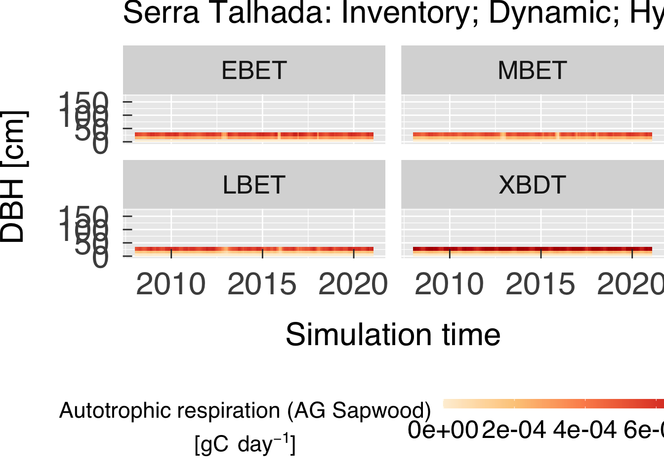
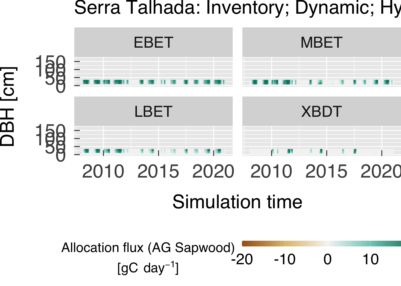

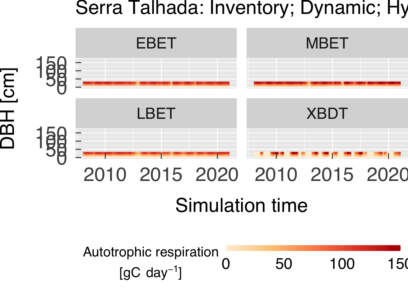
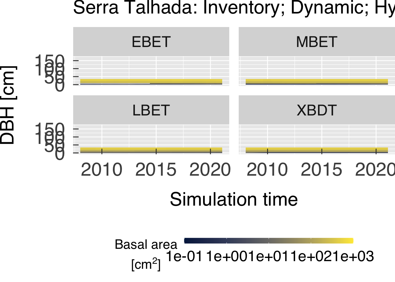
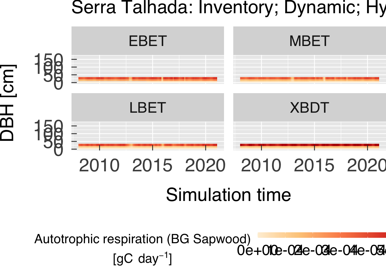


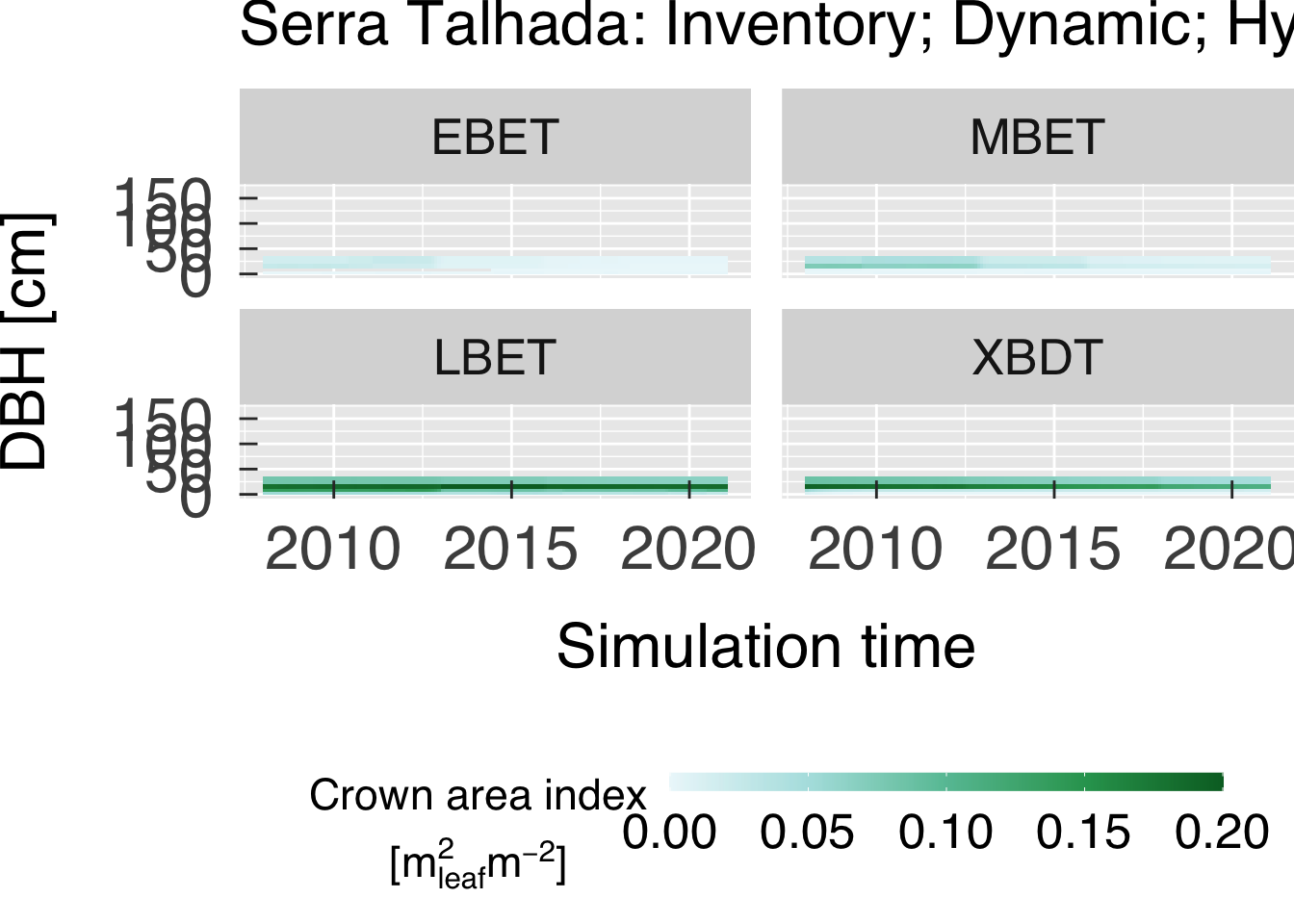
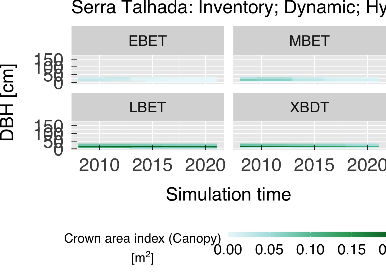
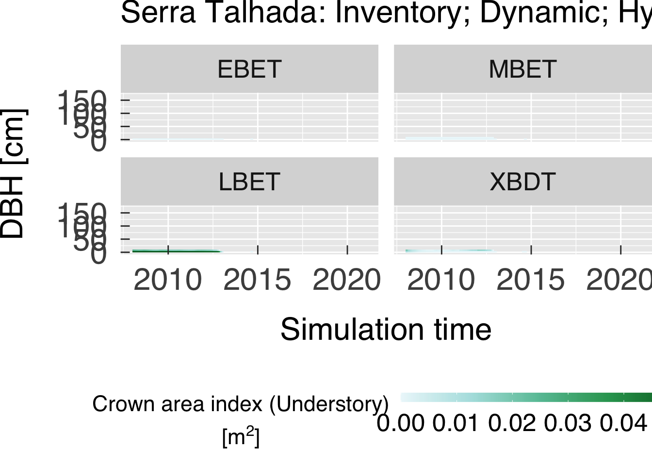
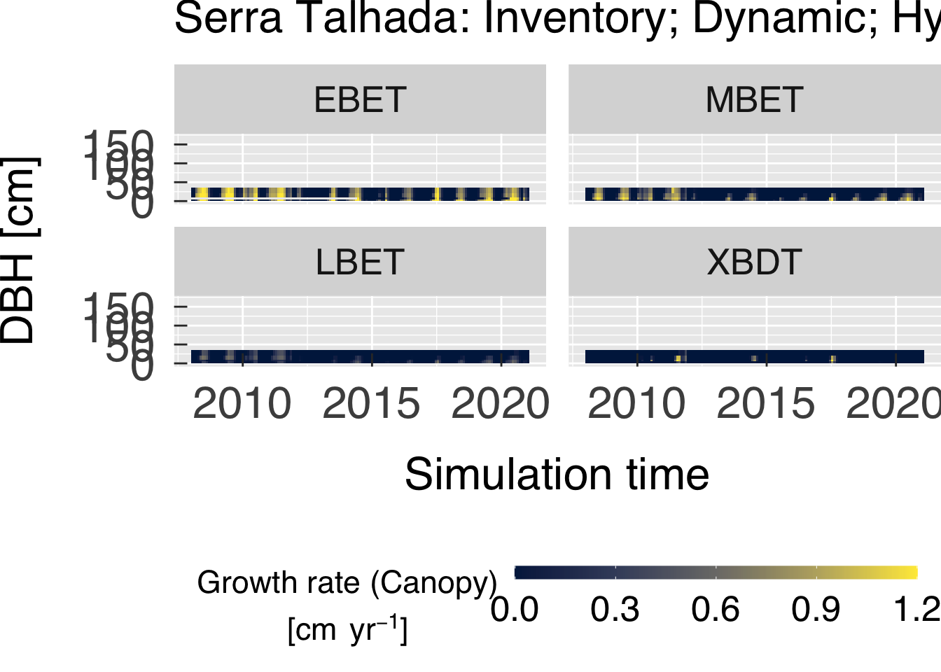
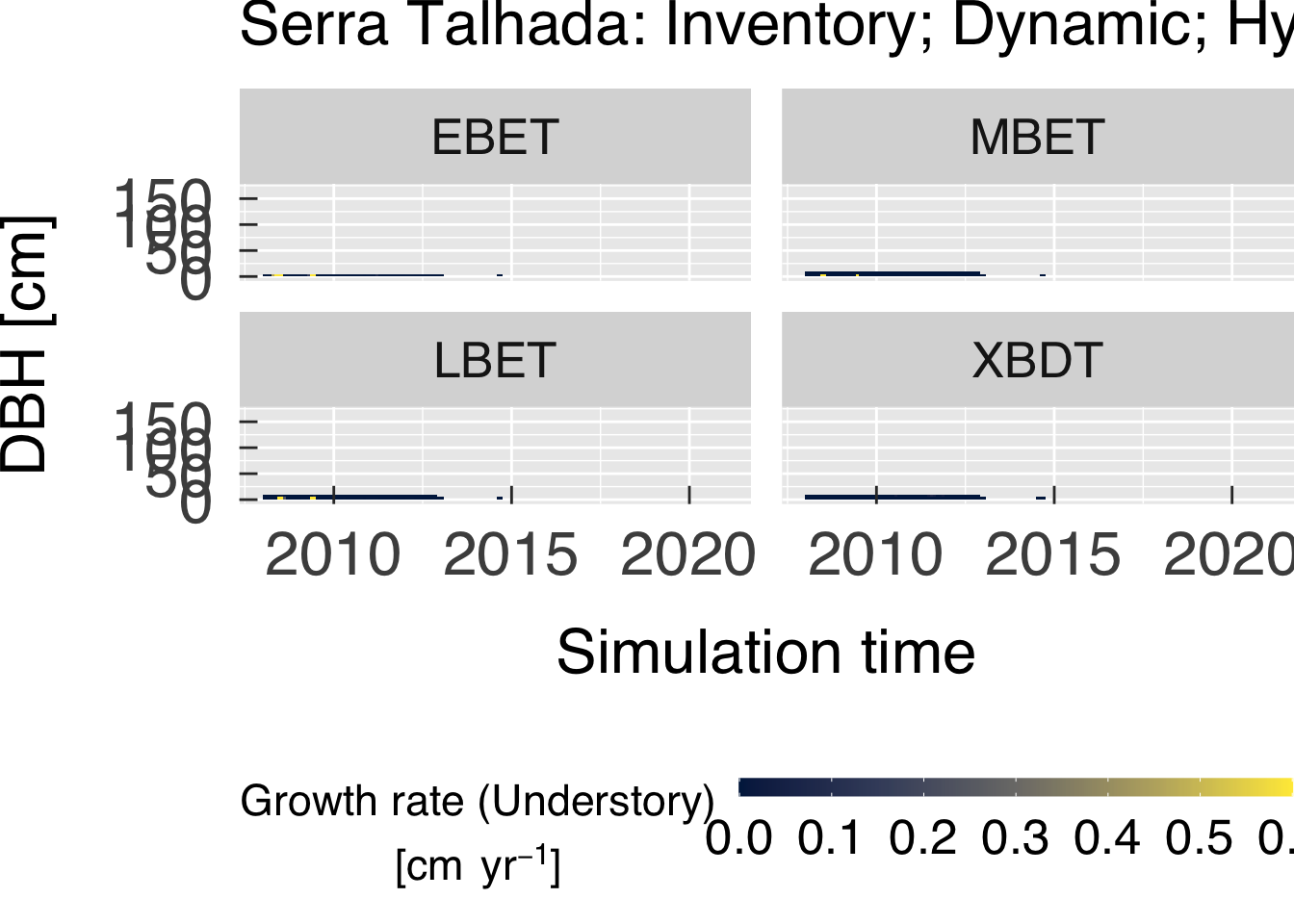
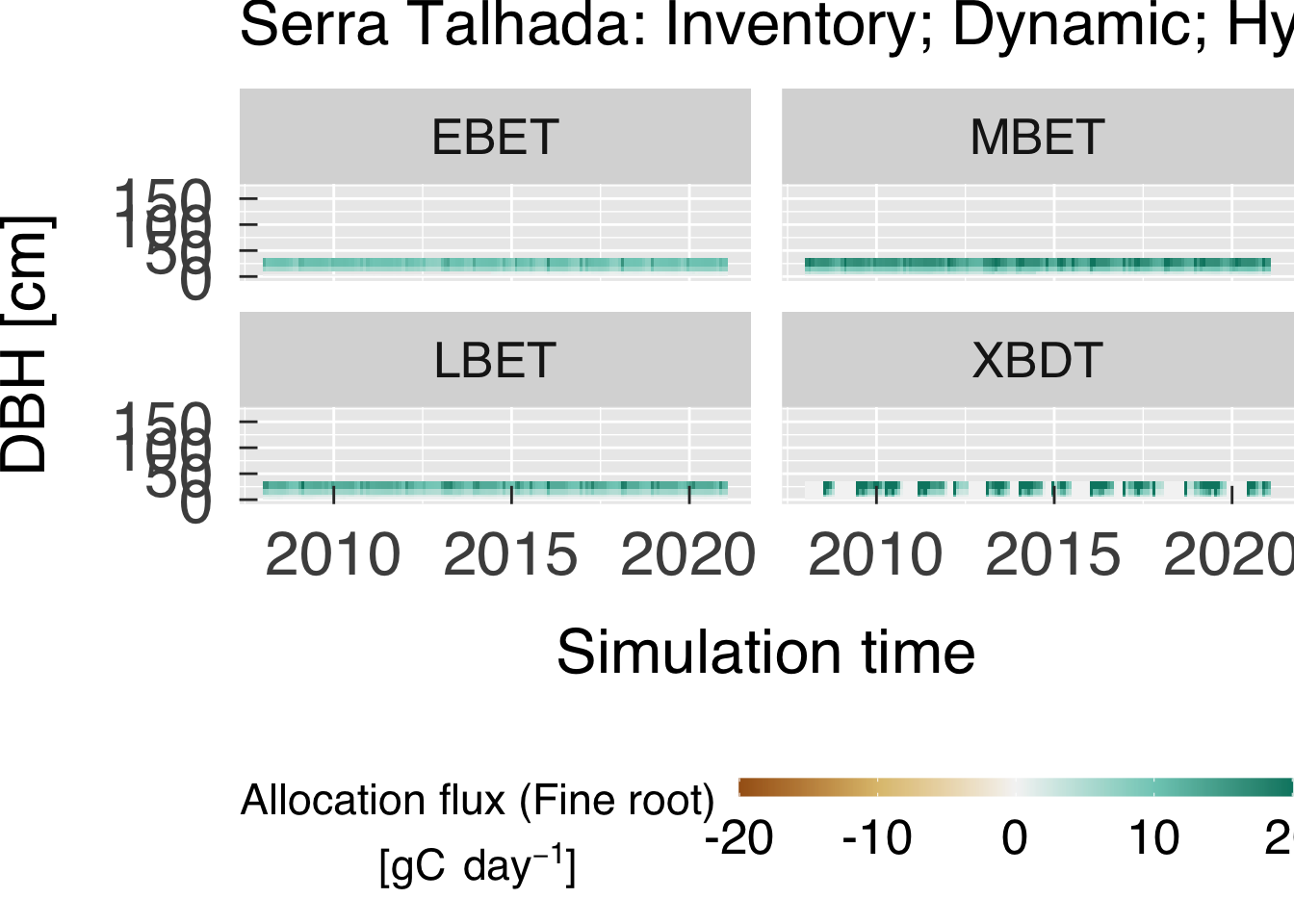
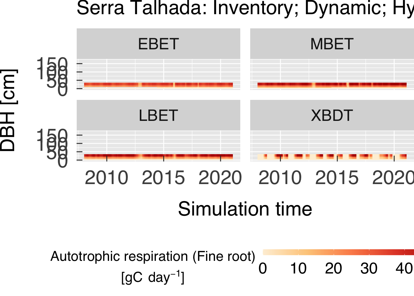
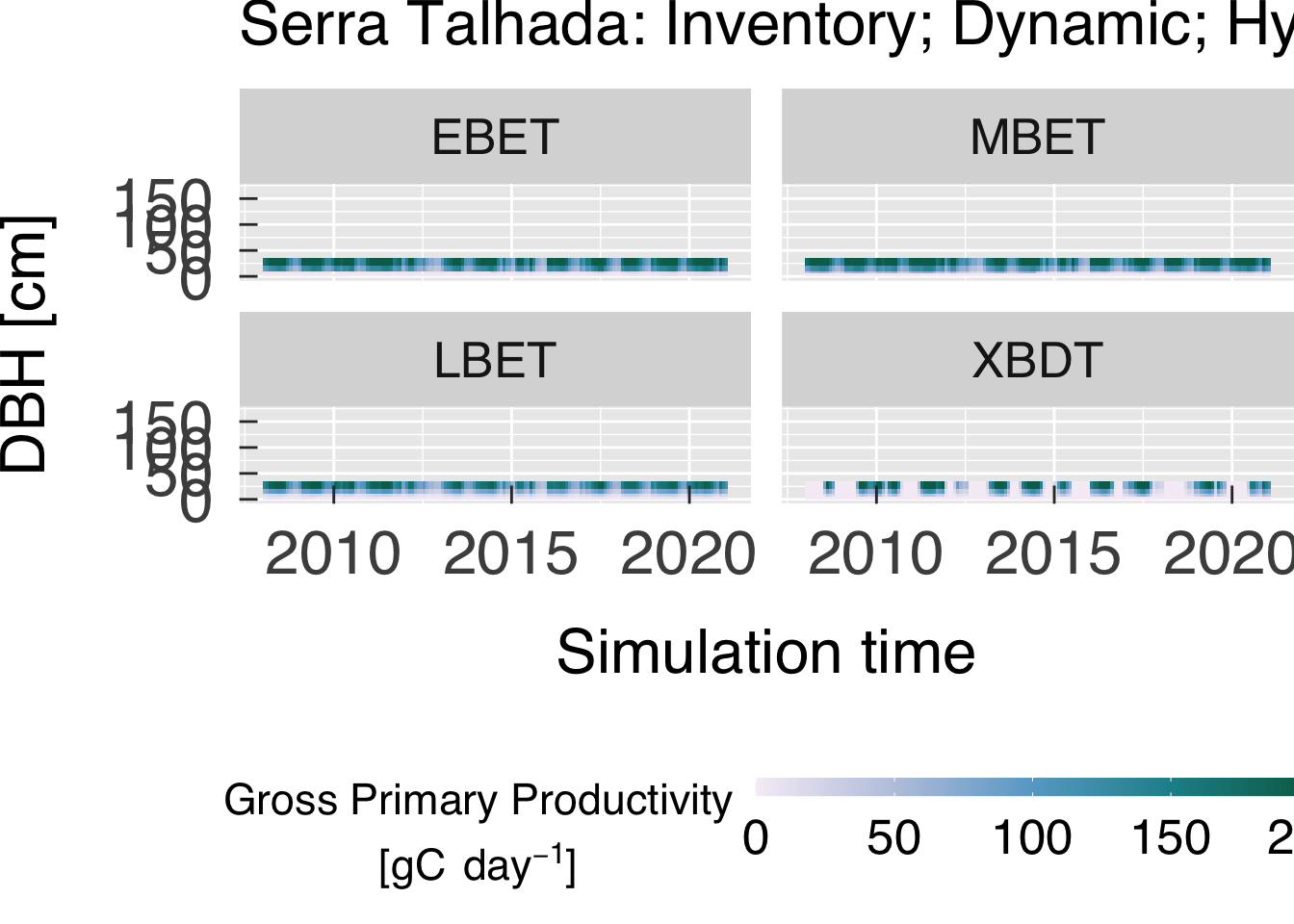
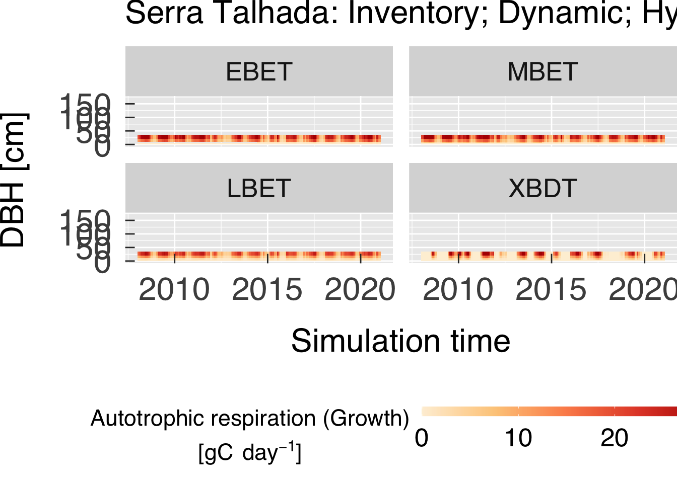
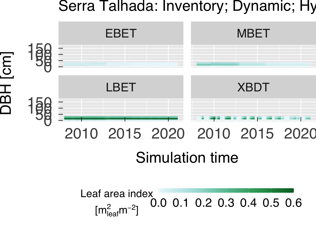
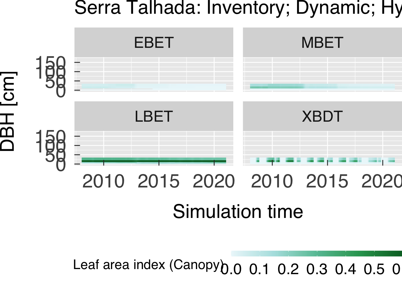
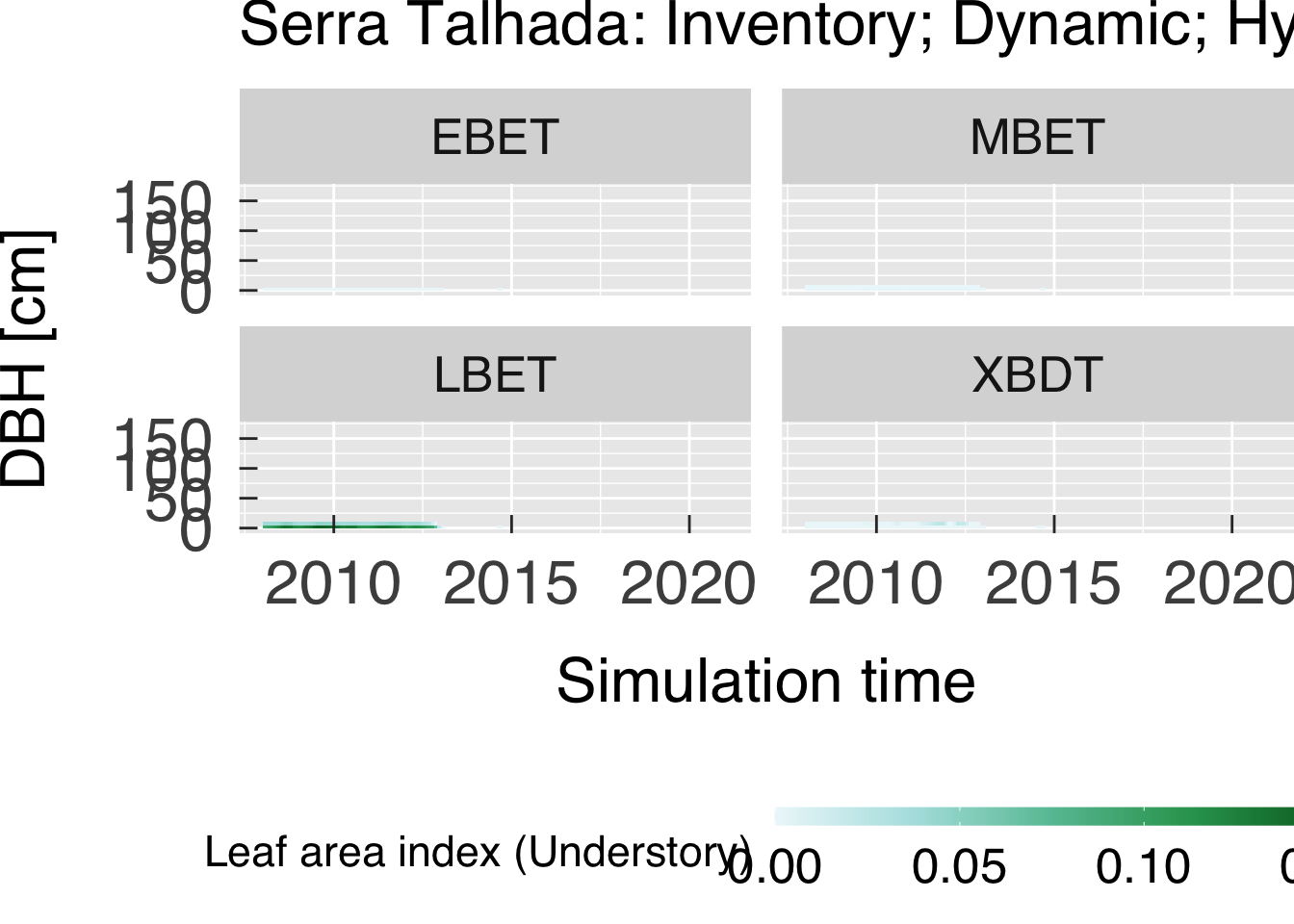
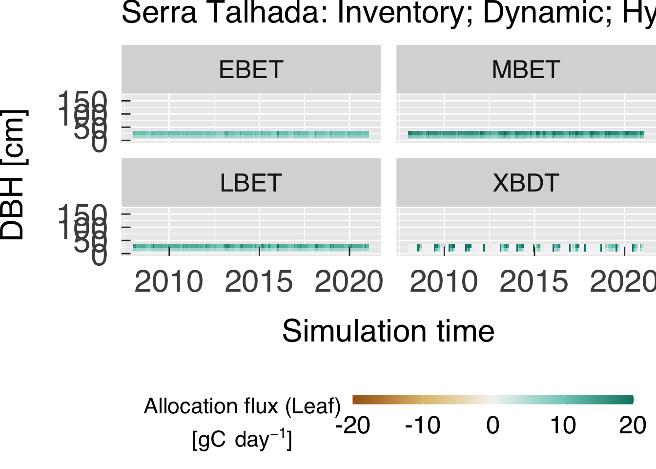
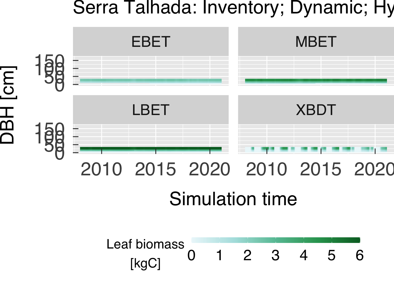
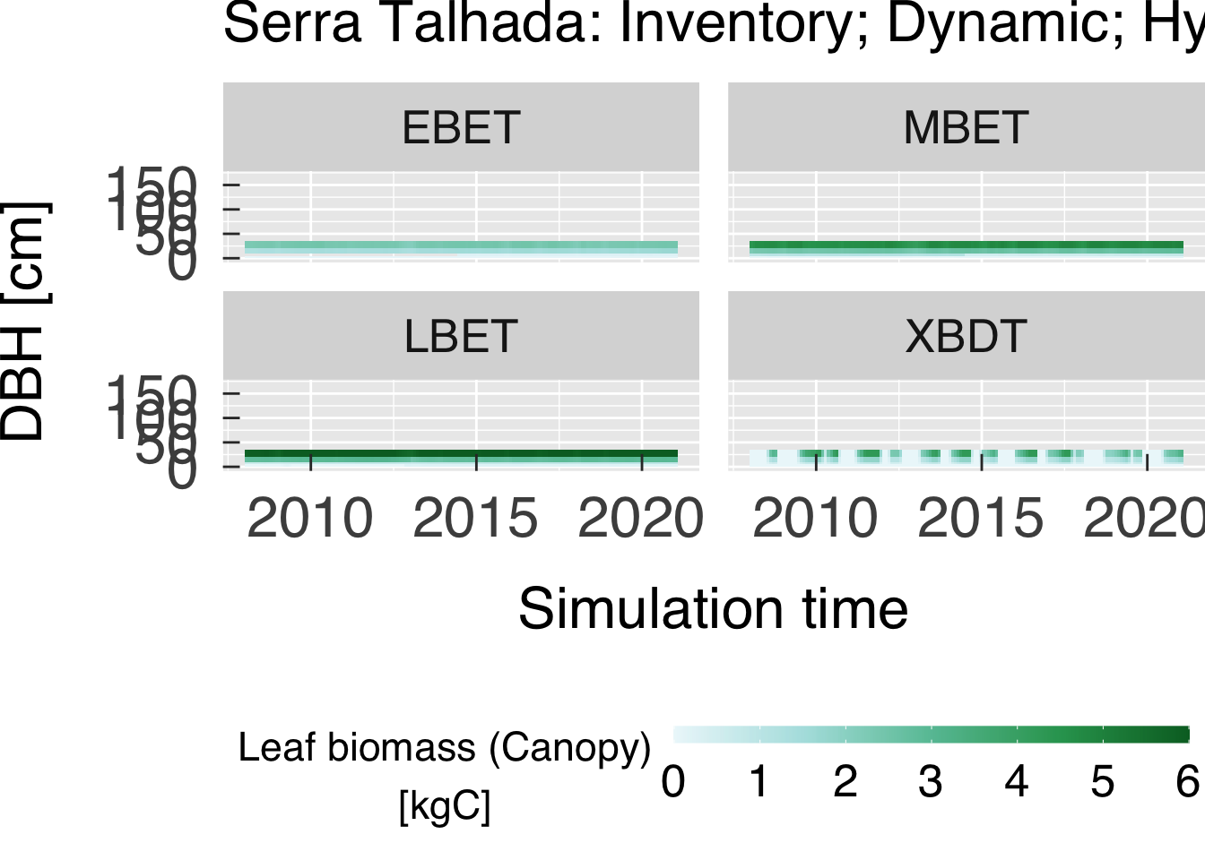
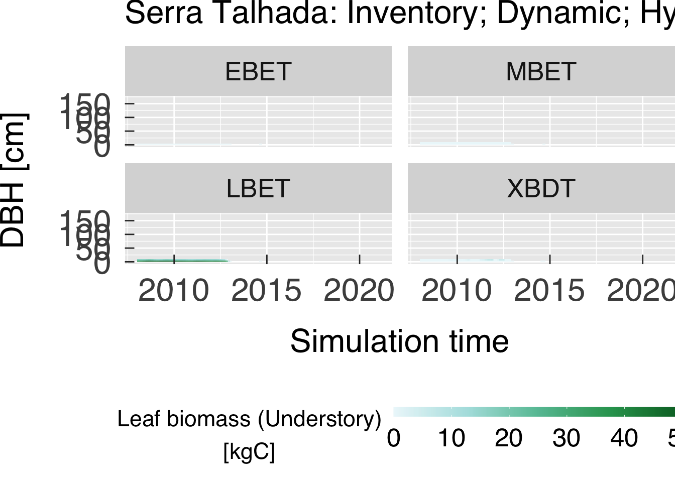
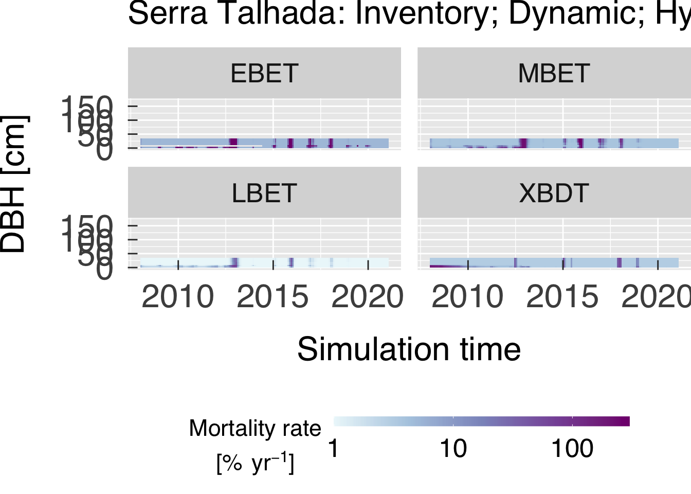
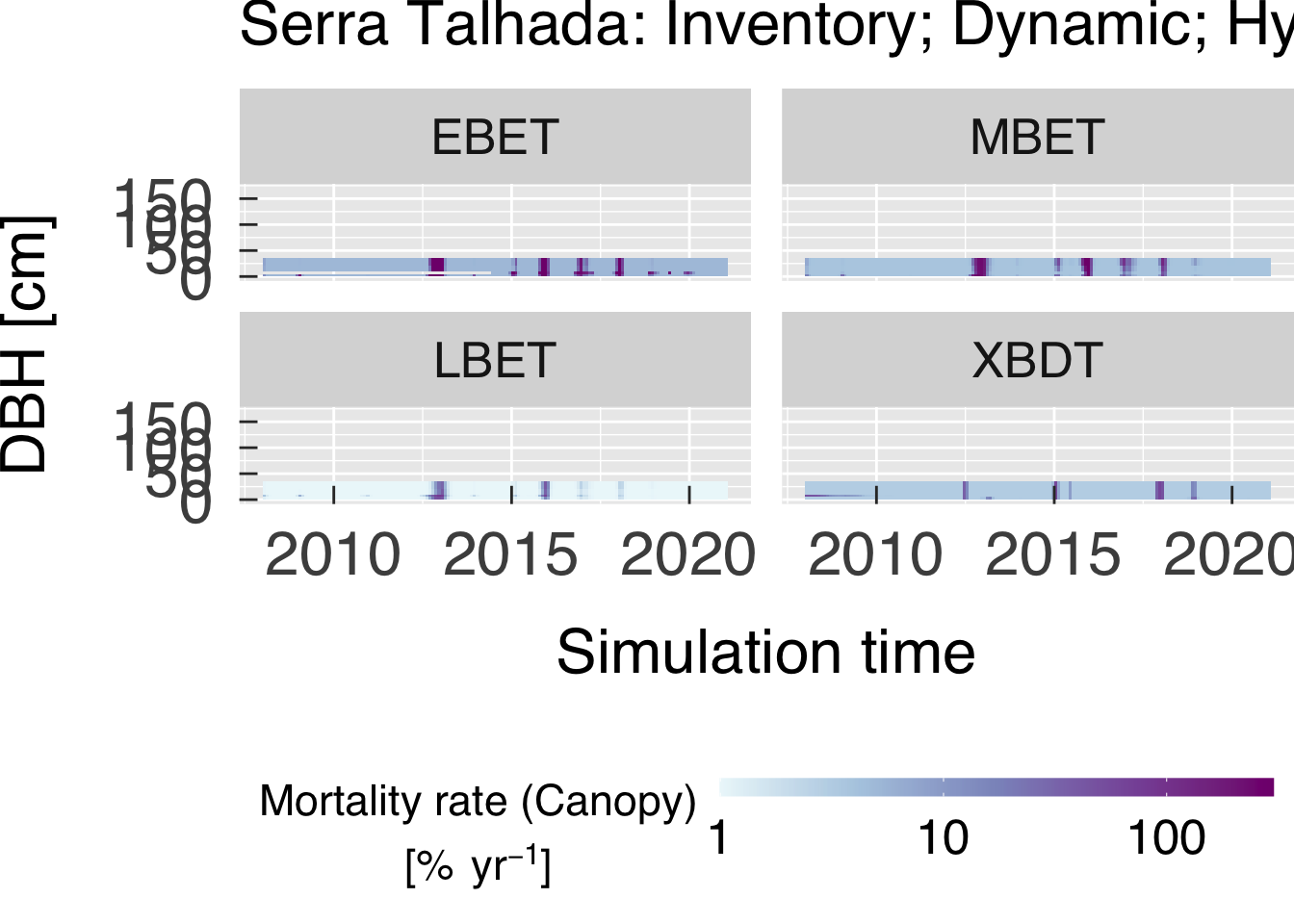
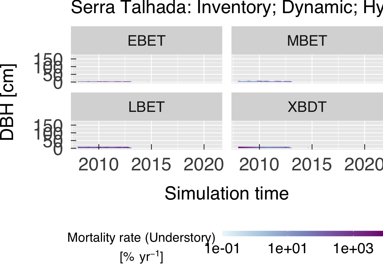
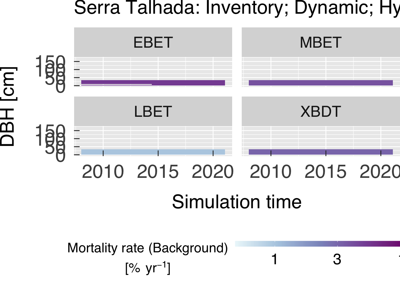
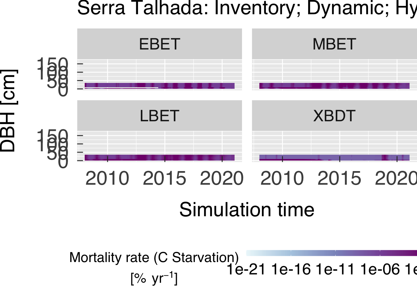
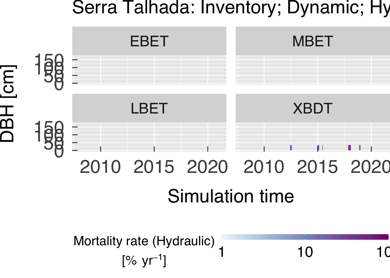
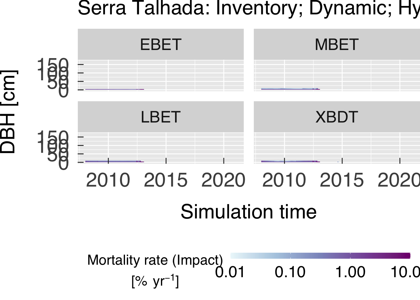
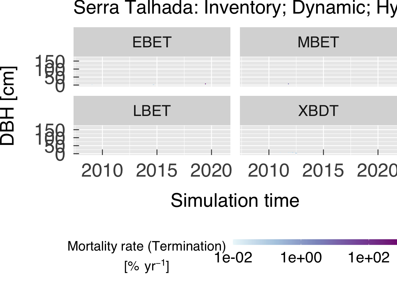
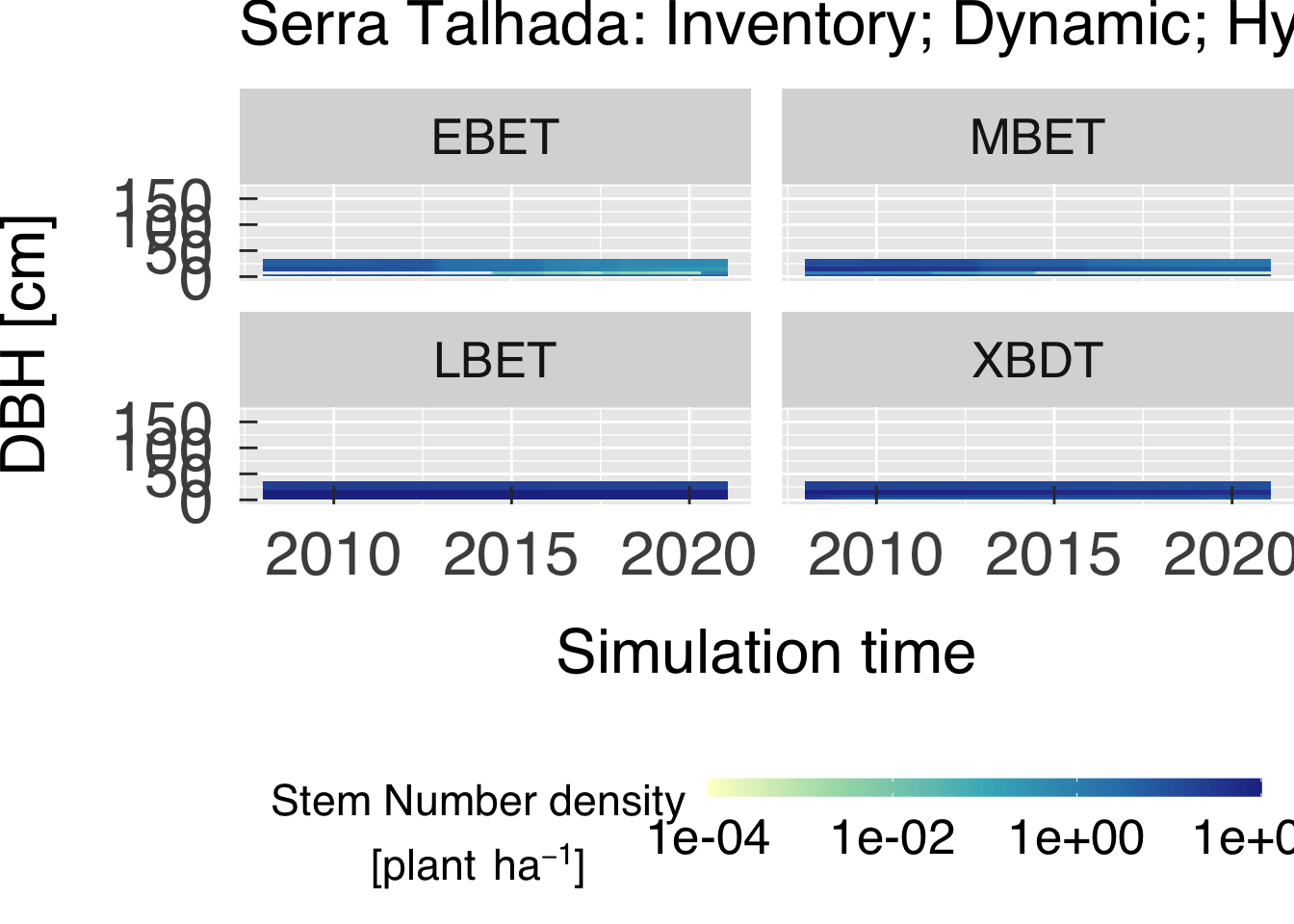
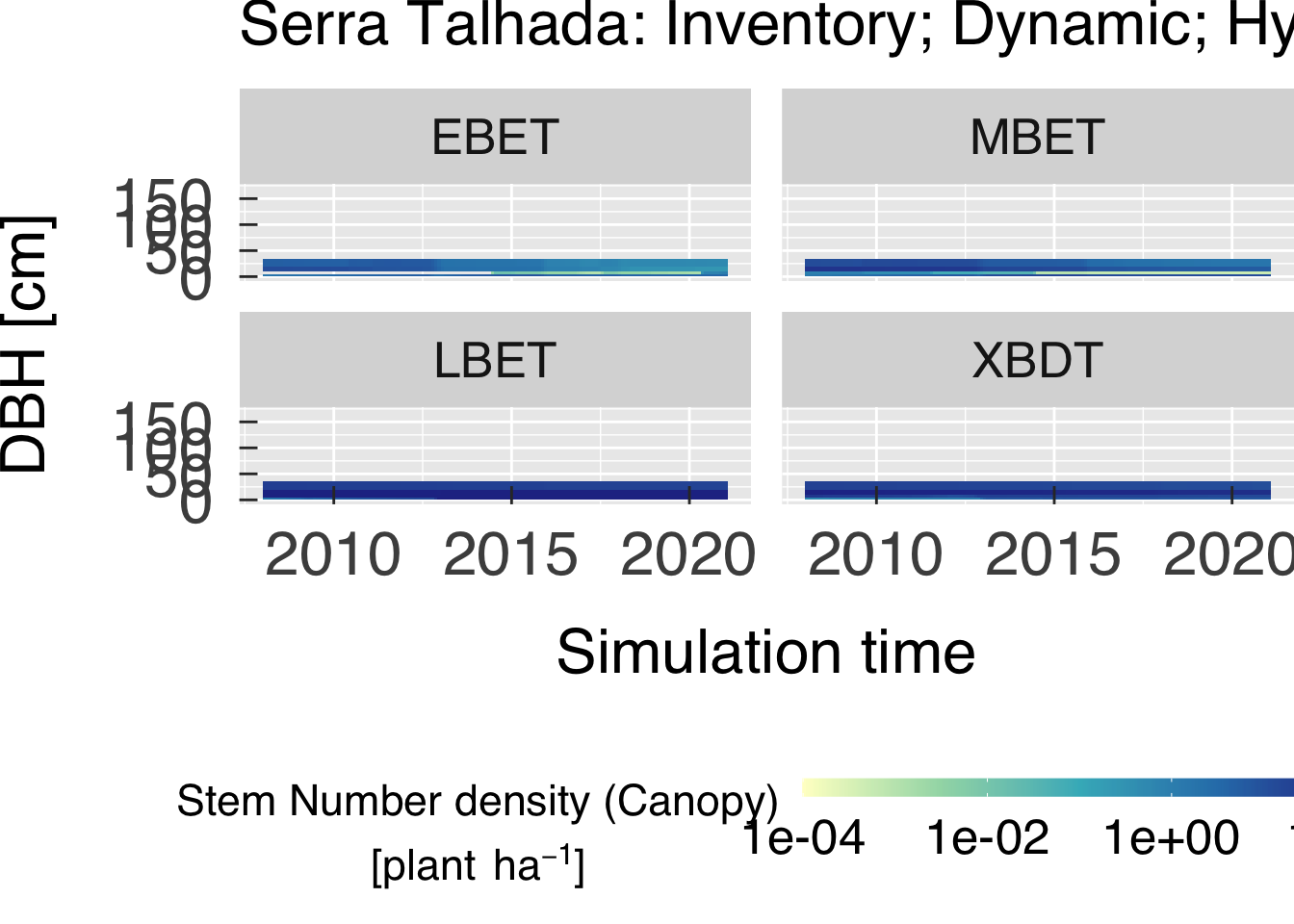
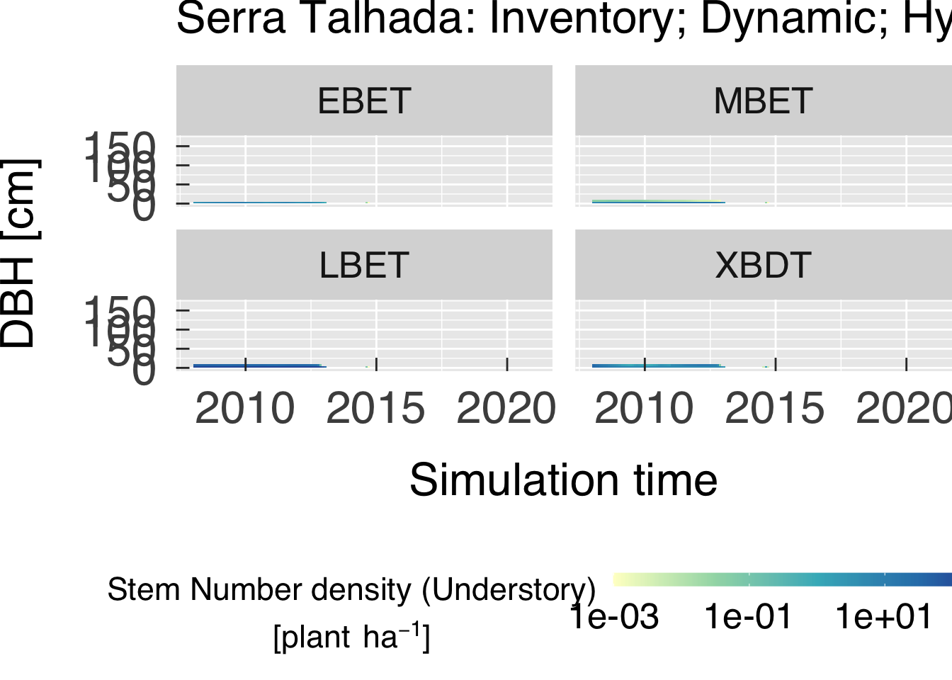
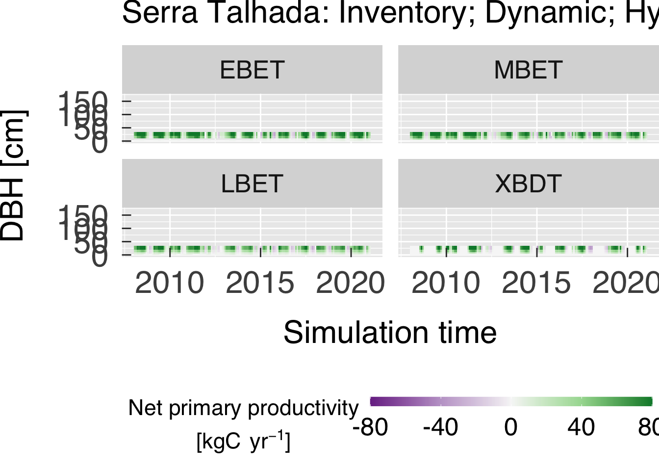
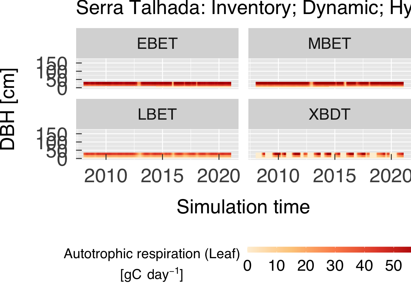
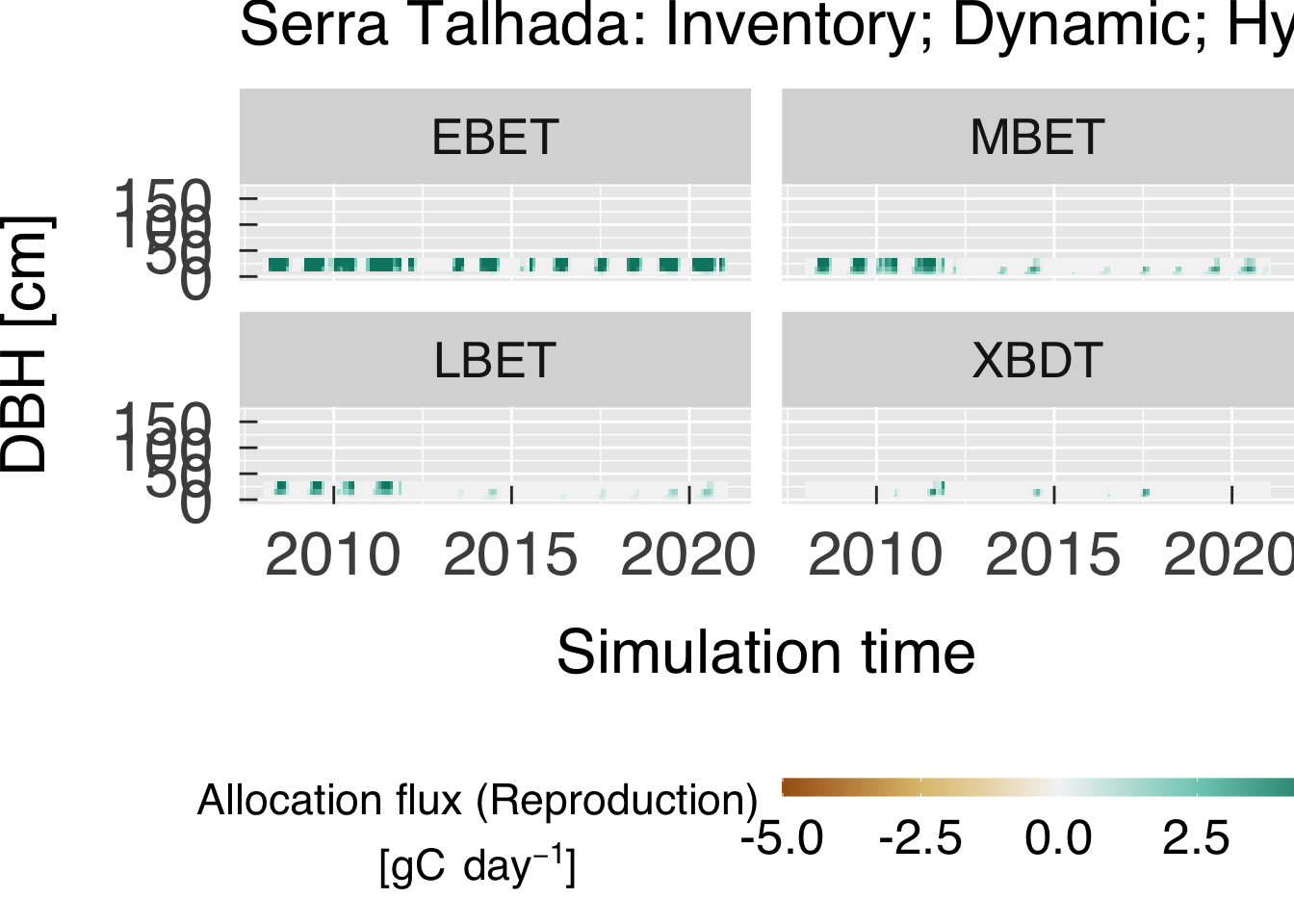
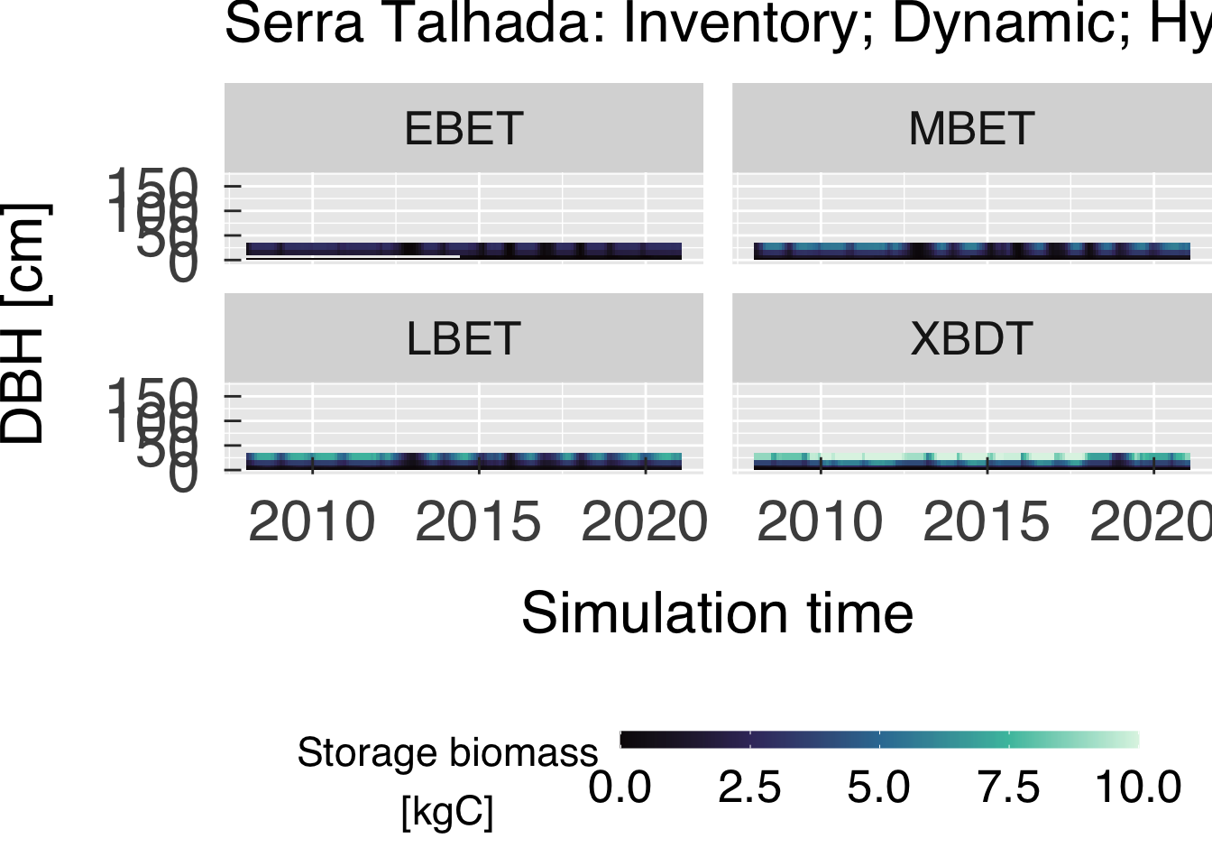
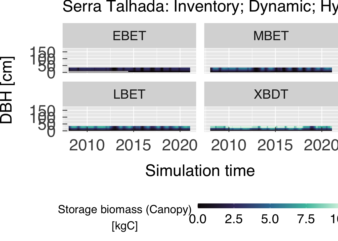
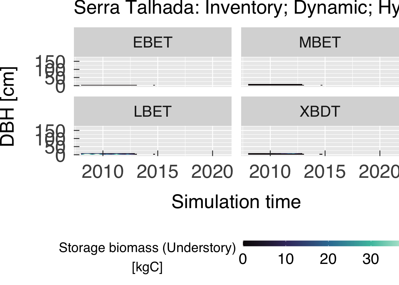
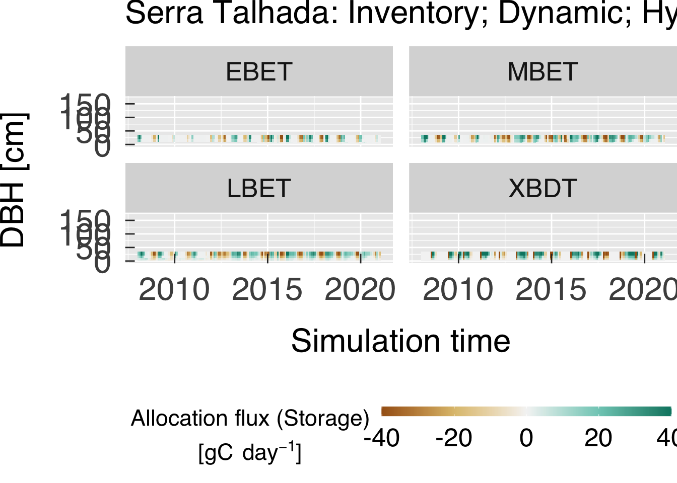
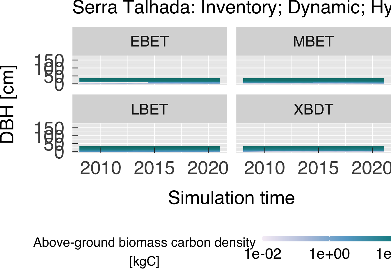
Plot theme time series:
cat0(" + Plot time series of thematically linked variables.")

gg_theme   = list()
for (th in sequence(ntstheme)){
  # Match variables.
  th_thnam  = tstheme$thnam  [th]
  th_thdesc = tstheme$thdesc [th]
  th_thunit = tstheme$thunit [th]
  th_stack  = tstheme$thstack[th]
  th_trans  = tstheme$trans  [th]
  th_vnames = tstheme$vnames [th]
  th_vcols  = tstheme$vcols  [th]

  # Split variables to include in this plot (plot only when all data are available).
  th_vlist   = c(unlist(strsplit(x=th_vnames,split="\\+")))
  th_match   = match(th_vlist,hlm1dvar$vnam)
  th_vdesc   = hlm1dvar$desc[th_match]
  th_labels  = parse(text=paste0("paste(",hlm1dvar$short[th_match],")"))
  n_th_vlist = length(th_vlist)


  # Proceed only if all variables exist in the output
  if (all(th_vlist %in% names(hlm1d))){
     # Title for legend
     cat0("   - ",th_thdesc,".")

     # Temporary data table. We convert the classes back to factor.
     thmelt       = hlm1d %>% select_at(th_vlist)
     thmelt$time  = tstamp
     thmelt       = melt( data          = thmelt
                        , id.vars       = "time"
                        , variable.name = "idvar"
                        , measure.vars  = th_vlist
                        , value.name    = th_thnam
                        )#end melt
     thmelt       = as_tibble(thmelt)
     thmelt$idvar = factor(as.integer(thmelt$idvar))

     # Find colours for theme plot.
     th_funcol   = try(match.fun(th_vcols),silent=TRUE)
     if ("try-error" %in% is(th_funcol)){
       th_colour = c(unlist(strsplit(x=th_vcols,split="\\+")))
     }else{
       th_colour = th_funcol(n=n_th_vlist)
     }#end if ("try-error %in% is(th_funcol))


     # Initialise plot (decide whether to plot lines or stacks).
     if (th_stack){
        gg_now = ggplot(data=thmelt,aes_string(x="time",y=th_thnam,group="idvar",fill="idvar"))
        gg_now = gg_now + scale_fill_manual(name=character(0),labels=th_labels,values=th_colour)
        gg_now = gg_now + geom_area(position="stack",show.legend = TRUE)
     }else{
        gg_now = ggplot(data=thmelt,aes_string(x="time",y=th_thnam,group="idvar",colour="idvar"))
        gg_now = gg_now + scale_colour_manual(name=character(0),labels=th_labels,values=th_colour)
        gg_now = gg_now + geom_line(lwd=1.0,show.legend = TRUE)
     }#end if (f_stack)
     gg_now = gg_now + labs(title=case_desc)
     gg_now = gg_now + scale_x_datetime(date_labels=gg_tfmt)
     gg_now = gg_now + scale_y_continuous(trans=th_trans,labels=label_number_auto())
     gg_now = gg_now + xlab("Simulation time")
     gg_now = gg_now + ylab(desc.unit(desc=th_thdesc,unit=untab[[th_thunit]],twolines=TRUE))
     gg_now = gg_now + theme_grey( base_size      = gg_ptsz
                                 , base_family    = "Helvetica"
                                 , base_line_size = 0.5
                                 , base_rect_size = 0.5
                                 )#end theme_grey
     gg_now = gg_now + theme( legend.position   = "bottom"
                            , axis.text.x       = element_text( size   = gg_ptsz
                                                              , margin = unit(rep(0.35,times=4),"cm")
                                                              )#end element_text
                            , axis.text.y       = element_text( size   = gg_ptsz
                                                              , margin = unit(rep(0.35,times=4),"cm")
                                                              )#end element_text
                            , axis.ticks.length = unit(-0.25,"cm")
                            , plot.title        = element_text( size = gg_ptsz)
                            )#end theme

     # Save plot.
     for (d in sequence(ndevice)){
        th_output = paste0(th_thnam,"-tstheme-",case_fpref,".",gg_device[d])
        dummy = ggsave( filename = th_output
                      , plot     = gg_now
                      , device   = gg_device[d]
                      , path     = tstheme_path
                      , width    = gg_width
                      , height   = gg_height
                      , units    = gg_units
                      , dpi      = gg_depth
                      )#end ggsave
     }#end for (o in sequence(nout))

     # Write plot settings to the list.
     gg_theme[[th_thnam]] = gg_now

  }#end if (all(th_vlist %in% names(hlm1d))))
}#end for (a in age_loop)


# If sought, plot images on screen
if (gg_screen) gg_theme