Reset session
Use this chunk to fully reset R.
# Unload all packages except for the R default ones
plist = names(sessionInfo()$otherPkgs)
if (length(plist) > 0){
   dummy = sapply(X=paste0("package:",plist),FUN=detach,character.only=TRUE,unload=TRUE)
}#end if (length(plist) > 0)


# Remove all variables
rm(list=ls())

# Reset warnings
options(warn=0)

# Close all plots
invisible(graphics.off())

# Clean up
invisible(gc())
Introduction.
This script seeks to establish trait trade-off relationships for
different plant functional groups.
Set paths and file names for input and output.
- home_path. The user home path.
- main_path. Main working directory
- util_path. The path with the additional utility
scripts (the full path of
RUtils).
- summ_path. Path for summaries by species, genus and
cluster.
- plot_path. The main output path for the simulation
plots.
- rdata_path. Output path for R objects (so we can
use it for comparisons.)
- br_state_shp. Shapefile with Brazilian states.
# Set useful paths and file names
home_path       = path.expand("~")
main_path       = file.path(home_path,"Data","TraitAllom_Workflow")
util_path       = file.path(main_path,"RUtils")
summ_path       = file.path(main_path,"TaxonSummary")
plot_path       = file.path(main_path,"Figures")
rdata_path      = file.path(main_path,"RData")
br_state_shp    = file.path(main_path,"BrazilianStatesMap","BrazilianStates.shp")
Settings for reloading or rerunning multiple steps of this script.
These are all logical variables, with TRUE meaning to
reload previous calculations, and FALSE meaning to
calculate the step again. If the RData file is not found, these
variables will be ignored.
- reload_SMA_trait. Reload the SMA fits for traits
(general)?
- reload_SMA_photo. Reload the SMA fits for traits
(photosynthesis traits)?
- reload_corr_trait. Reload the rank correlation
matrix (general)?
- reload_impute. Reload the imputed data sets?
- reload_cluster. Reload the cluster analysis.
reload_SMA_trait  = c(FALSE,TRUE)[2L]
reload_SMA_photo  = c(FALSE,TRUE)[2L]
reload_corr_trait = c(FALSE,TRUE)[2L]
reload_impute     = c(FALSE,TRUE)[2L]
reload_cluster    = c(FALSE,TRUE)[2L]
This flag defines whether to exclude observations from traits that
show high light plasticity but were not collected from sunny leaves. If
plastic_sun_only=TRUE, the code will exclude traits that
are considered photo-plastic, unless there is high likelihood that the
trait measurements used leaves in full sun (the exception being shrubs
living in closed canopy habitats, which are assumed to be understorey
specialists). If plastic_sun_only=FALSE, the code will keep
all trait measurements.
plastic_sun_only = c(FALSE,TRUE)[2L]
This flag defines the levels of experiments to be included (missing
values are always assumed natural and thus included). -
0. Control data sets (i.e., those without treatment in
treatment experiments) - 1. Minor treatments (i.e.,
fences or logging, where the changes in environment are unlikely to
affect traits beyond what could normally occur in the landscape) -
2. Temperature treatments (warming / cooling). -
3. Water treatments (droughts, irrigation) -
4. Light treatments (lamps, shades) -
5. \(\mathrm{CO}_2\)
experiments (enhancement, removal). - 6. Nutrient
experiments (fertilisation, suppression). - 7. Other
experiments (ozone, pesticides, multiple factors).
If use_treat_level=integer(0L), then only data from
non-treatment studies will be considered. We advise to include at least
level 0, as they are often equivalent to non-treatment studies. If
use_treat_level=NA_integer_, then the flag will be ignored,
meaning that treatment data will be all considered.
use_treat_level = c(0L,1L) # Which treatment levels to include in data analysis
This flag defines whether to keep only woody plants, and how strict
we should be about it. Possible values are:
- tree_only. Only trees (sensu stricto) are included.
This will exclude shrubs, lianas, hemiepiphytes and tree-like forms
(e.g., palms, yucca “trees”).
- woody_ss_free. All free-standing woody plants
(sensu stricto) are included. This will include trees and shrubs, but
exclude lianas, hemiepiphytes, and tree-like forms.
- woody_ss_all. All woody plants (sensu stricto) are
included. This will include trees, lianas, shrubs and hemiepiphytes, but
exclude tree-like forms.Summ
- woody_sl_free. All free-standing woody plants
(sensu lato) are included. This will include trees, shrubs and tree-like
forms, but exclude lianas and hemiepiphytes.
- woody_sl_all. All woody plants (sensu lato) are
included. This will include trees, lianas, shrubs, palms and
hemiepiphytes.
- all_plants. All plants will be retained.
use_woody_level = c("tree_only","woody_ss_free","woody_ss_all","woody_sl_free","woody_sl_all","all_plants")[2L]
The following block defines some settings for the standardised major
axis for most traits and photosynthesis traits:
xsma_TraitID. Variable to be used as the X axis
of the SMA fit for most traits. This must be a trait ID that matches one
of the traits listed in try_trait, defined in the trait
file list (trait_file) and loaded from file
rdata_TidyTRY.
xphoto_TraitID. Variable to be used as the X
axis of the SMA fits for photosynthesis. This must be a trait ID that
matches one of the traits listed in try_trait, defined in
the trait file list (trait_file) and loaded from file
rdata_TidyTRY.
n_violin_min. Minimum number of valid points to
consider for violin diagrams.
n_fit_min. Minimum number of valid points to
consider for SMA fits.
n_predict. Number of points used along the trait
span to make the fitted curve.
n_boot. Number of bootstrap iterations for
building confidence bands for SMA models.
SMA_ConfInt. Confidence range for the SMA
models.
SMA_CorrMin. Minimum (absolute) correlation to
fit SMA models. This is needed because at very low correlations, the
slope of the SMA fit may flip from negative to positive in between
bootstrap samples and cause very odd confidence ranges. These fits are
not significant, so we skip them altogether.
SMA_Robust. Use robust approach for fitting SMA
(TRUE|FALSE). Robust fitting is better, but it
takes much longer because of the bootstrap uncertainty quantification.
Set this to FALSE when testing, so it saves time, and set
this to TRUE when producing the final results.
SMA_MaxIter. Maximum number of iterations for
confidence interval. This is needed especially when SMA_Robust is
FALSE, because the default SMA is not robust to outliers,
and confidence ranges may be outside the expected value. This typically
occurs in poor model fittings.
use_lifeclass. Which life-form/phylogenetic
level was used to subset the original data set. Options are:
"FlowerTrees". Trees, classes Magnoliopsida and
Liliopsida (flowering plants)."Shrubs". Shrubs"Grasses". Grasses/Herbs"FlowerPlants". All life forms, classes Magnoliopsida
and Liliopsida"Pinopsida". Conifers (class Pinopsida), all life
forms"SeedPlants". Seed plants, all life forms: classes
Cycadopsida, Ginkgoopsida, Gnetopsida, Liliopsida, Magnoliopsida and
Pinopsida."Plantae". All plants
use_realm. Which realm was used to subset the
original data set. Current options are:
"NeoTropical". South and Central America"PanTropical". All continents."AfricaTropical". Africa"AsiaTropical". Asia"WestUS". Western US
fit_taxon. Which taxonomic level of detail to
use for SMA analyses? Options are:
"Individual". Treat each individual independently (only
individuals with measurements of traits in both axes will be
included)."Species". Find trait averages for species then compute
SMA (useful for somewhat sparse measurements)."Genus". Find trait averages for genus then compute SMA
(useful for very sparse measurements).
# Variable to use as X axis for trait SMA analyses?
xsma_TraitID    = c(SLA=3117L,wood_dens=4L,leaf_c2n=146L,leaf_n_area=50L)[1L]

# Variable to use as X axis for trait SMA analyses of photosynthesis traits?
xphoto_TraitID  = c(a_amax=53L,a_vcmax=186L,a_jmax=269L,m_amax=40L,m_vcmax=185L,m_jmax=270L)[2L]

# Minimum number for plotting violins
n_violin_min    = 10L

# Minimum number of points for SMA fitting.
n_fit_min       = 20L

# Number of points to build prediction curve.
n_predict       = 200L

# Number of bootstrap iterations
n_boot          = 1000L

# Confidence range for SMA models and correlation tests
SMA_ConfInt     = 0.95

# Minimum absolute correlation to fit the SMA model
SMA_AbsCorrMin  = 10^(-0.5)

# Use robust fitting for SMA?
SMA_Robust      = FALSE

# How many attempts for bootstrapping before giving up?
SMA_MaxIter     = 10L

# Life-form/phylogenetic level to use for SMA analyses.
use_lifeclass  = c("FlowerTrees","Shrubs","Grasses","FlowerPlants","Pinopsida","SeedPlants","Plantae")[4L]

# Realm to use for SMA analyses.
use_realm  = c("NeoTropical","PanTropical", "AfricaTropical", "AsiaTropical", "WestUS")[1L]

# Taxonomic level of detail for SMA analyses.
fit_taxon = c("Individual","Species","Genus")[2L]
Settings for Kendall correlation table.
- n_kendall_min. This is the minimum number of valid
pairs of variables for computing correlation.
- pmax_kendall_show. Maximum p-value for which
correlations are written to the CSV file.
n_kendall_min     = 30L   # Minimum number of data pairs for Kendall correlation.
pmax_kendall_show = 0.001 # Maximum correlation reported in the CSV file.
Settings for the Imputation, Cluster Analysis and Principal Component
Analysis:
- impute_cluster_test. Flag to decide whether to run
the code in test mode. If
TRUE, this will reduce the number
of Monte Carlo iterations to 10, halt the code after running the cluster
analysis and skip saving the imputation and cluster analysis RData
objects so the code can be tested again. When running the actual
analyses, make sure this is set to FALSE.
- n_row_numtrait_impute. For each entry (row), we
check whether the trait has a sufficient number of numeric
(non-categorical) traits to be included in imputation, and analyses that
depend upon the imputed table.
- f_col_trait_impute. For each column (trait), we
check whether the trait has sufficient valid data relative to the most
abundant numeric trait. Only those traits (numeric or categorical) that
exceed this threshold will be considered for imputation and subsequent
analyses (cluster analysis, PCA, etc.). This is provided as a
fraction.
- f_var_min_impute. For each column (trait), we check
whether the trait has sufficient variability to be included. For numeric
traits, variability is defined as standard deviation divided by the mean
of absolute values (to get the mean magnitude of trait values and not
worry about the sign or when the mean is close to zero). For categorical
traits, variability isd defined as evenness.
- rseed_impute. This is used to define the seed for
random numbers ahead of the imputation, to ensure reproducibility. If
set to
NA_integer_, the code will use time for setting the
seed, making it truly random.
- cluster_kmin. Minimum number of clusters to
consider (when seeking the optimum number of clusters)
- cluster_kmax. Maximum number of clusters to
consider (when seeking the optimum number of clusters)
- cluster_kfix. A number of clusters to be saved
regardless of the optimum. It must be between
cluster_kmin
and cluster_kmax. This is used depending on how
cluster_method is set.
- min_weight_cluster. Weighting threshold below which
traits are ignored in the cluster analysis
- rseed_cluster. This is used to define the seed for
random numbers ahead of the cluster analysis standard error, to ensure
reproducibility. If set to
NA_integer_, the code will use
time for setting the seed, making it truly random.
- n_mcarlo_cluster. Number of Monte Carlo iterations
to produce standard error for the gap statistics. Higher numbers yield
to more robust estimates, but this step takes a lot of time.
- method_gap_maxSE. Which method to use for selecting
the maximum gap statistics. This must be one of the options for argument
method in function clusGap::maxSE.
- cluster_method. Which method to use for selecting
the optimum number of clusters. Current options are “sil” (for
silhouette), “gap” (for gap statistics) or “fix” for a fixed number of
clusters (as set by
cluster_kfix. The script always
calculates both the silhouette and the gap stastitics, but the default
method is the one applied for subsequent analyses.
- n_pca_min. This is the minimum number of valid
points for running a PCA (after imputation).
# Run imputation and cluster analyses in test mode?
impute_cluster_test = c(FALSE,TRUE)[1L]

# Minimum number of numeric traits for keeping the entry for imputation. This avoids keeping plants for which we only have a few traits
n_row_numtrait_impute = 3L

# Minimum fraction of complete observations (relative to the most abundant numeric trait) for being considered in the imputation
f_col_trait_impute = 1./6.

# Minimum variability of the variable to be included in the imputation. Variability is sd(x)/mean(abs(x)) for numeric traits and
#    evenness for categorical traits (including ordered, integers, logical variables, and characters).
f_var_min_impute = 0.01

# Random seed for the imputation analysis (so results are reproducible)
rseed_impute = 6L

# Select the minimum and maximum number of clusters to consider.
cluster_kmin = 3L
cluster_kmax = 20L
cluster_kfix = 4L

# Minimum weight (first guess) below which the traits will be disregarded for cluster analysis
min_weight_cluster = 1./6.

# Random seed for the cluster analysis (so results are reproducible)
rseed_cluster = 12L

# Number of Monte Carlo iterations (for gap statistics standard error)
n_mcarlo_cluster = 100L

# Method for maximum gap statistics whilst accounting for standard error. See maxSE help for details.
method_gap_maxSE = c("firstSEmax","Tibs2001SEmax","globalSEmax","firstmax", "globalmax")[5L]

# Method to be used for selecting the optimum number of clusters.
cluster_method = c("sil","gap","fix")[2L]

# Minimum number of valid points for running a PCA.
n_pca_min = 500L
The following tibble object sets colours and shapes for categorical
traits that will be used for analysis. Only the classes included in this
list will be displayed. This tibble should contain the following
columns:
- TraitID. The trait ID to which the categories
correspond to. This must be the same ID used by TRY. Additionally, you
should include two rows with TraitID set no
NA_integer_.
These rows will have special settings for unknown classes and for the
global model.
- Class. This is the new simplified class for plots
and analyses. In case you want to direct multiple original classes to
fewer simplified classes, use the same name in this column multiple
times. For the special rows, set one of them to “UKN” and the other to
“ALL”, for entries that could not be classified and one for the full
model.
- TRYClass. The input class categories from TRY,
after the primary harmonisation by script TidyTraitAllomDB.Rmd.
- Colour. Colour to be used for this class. If
multiple
TRYClass entries point to the same
Class for a given trait ID, only the first value of
Colour for that Class will be considered.
- Symbol. Symbol to be used for this class. If
multiple
TRYClass entries point to the same
Class for a given trait ID, only the first value of
Symbol for that Class will be considered.
- XYUse. Which column to use for scatter plots.
Options are
"Colour", "Symbol", or
NA_character_. Make sure the values are the same for all
rows belonging to the same TraitID, and that both "Colour"
and "Symbol" are not used for two or more traits.
# Phenology information
CategInfo = tidyr::tribble( ~TraitID, ~Class, ~TRYClass                     ,   ~Colour, ~Symbol, ~XYUse       , ~Order
                          ,         22L,   "C3", "C3"                       , "#007E89",     17L, NA_character_, NA_integer_
                          ,         22L,   "C4", "C4"                       , "#FCA2AE",      5L, NA_character_, NA_integer_
                          ,         22L,  "CAM", "CAM"                      , "#B6899C",      8L, NA_character_, NA_integer_
                          ,         28L,  "ZOO", "Zoochory"                 , "#AED5E3",      9L, NA_character_, NA_integer_
                          ,         28L,  "ZOO", "Ornithochory"             , "#AED5E3",      9L, NA_character_, NA_integer_
                          ,         28L,  "ZOO", "Mammalochory"             , "#AED5E3",      9L, NA_character_, NA_integer_
                          ,         28L,  "AUT", "Autochory"                , "#FCA2AE",     13L, NA_character_, NA_integer_
                          ,         28L,  "HYD", "Hydrochory"               , "#008B96",     18L, NA_character_, NA_integer_
                          ,         28L,  "ANE", "Anemochory"               , "#E72521",     16L, NA_character_, NA_integer_
                          ,         37L,  "EVG", "Evergreen"                , "#008B96",     18L, "Colour"     , 1L
                          ,         37L,  "BVD", "Brevi-deciduous"          , "#AED5E3",     13L, "Colour"     , 2L
                          ,         37L,  "SMD", "Semi-deciduous"           , "#FDBF6F",      9L, "Colour"     , 3L
                          ,         37L,  "DRD", "Deciduous (not specified)", "#E72521",     16L, "Colour"     , 4L
                          ,         38L,  "NWD", "Non-woody"                , "#008B96",     18L, NA_character_, 1L
                          ,         38L,  "SWD", "Semi-woody"               , "#7570B3",      9L, NA_character_, 2L
                          ,         38L,  "WDY", "Woody"                    , "#E72521",     16L, NA_character_, 3L
                          ,         42L,  "HBG", "Grass-Herb"               , "#E6AB02",      4L, "Symbol"     , NA_integer_
                          ,         42L,  "LIA", "Liana"                    , "#7570B3",     17L, "Symbol"     , NA_integer_
                          ,         42L,  "PLM", "Palm"                     , "#66A61E",     18L, "Symbol"     , NA_integer_
                          ,         42L,  "SHB", "Shrub"                    , "#D95F02",      8L, "Symbol"     , NA_integer_
                          ,         42L,  "TRE", "Tree"                     , "#1B9E77",     16L, "Symbol"     , NA_integer_
                          ,         42L,  "VNE", "Vine"                     , "#222222",     13L, "Symbol"     , NA_integer_
                          ,         42L,  "XPH", "Xerophyte"                , "#E7298A",      6L, "Symbol"     , NA_integer_
                          ,        197L,  "BDT", "Broadleaf Deciduous Tree" , "#1B9E77",     16L, NA_character_, NA_integer_
                          ,        197L,  "BET", "Broadleaf Evergreen Tree" , "#66C2A5",     10L, NA_character_, NA_integer_
                          ,        197L,  "C3G", "C3 Grass"                 , "#E6AB02",      3L, NA_character_, NA_integer_
                          ,        197L,  "C4G", "C4 Grass"                 , "#FC8D62",      4L, NA_character_, NA_integer_
                          ,        197L,  "ESH", "Evergreen Shrub"          , "#7570B3",      2L, NA_character_, NA_integer_
                          , NA_integer_,  "UKN", "Unknown"                  , "#AAAAAA",      0L, NA_character_, NA_integer_
                          , NA_integer_,  "ALL", "All data"                 , "#161616",     15L, NA_character_, NA_integer_
                          )#end tribble
CntCategInfo = nrow(CategInfo)
Set up some flags to skip plotting sets of figures if they are not
needed
plot_violin         = c(FALSE,TRUE)[1L] # Violin plots for different groups?
plot_abund_map      = c(FALSE,TRUE)[2L] # Maps with trait abundance?
plot_stat_cluster   = c(FALSE,TRUE)[2L] # Plot statistics for generating the optimal number of clusters?
plot_wgt_cluster    = c(FALSE,TRUE)[2L] # Plot weights for cluster analysis?
plot_pca_cluster    = c(FALSE,TRUE)[2L] # Plot PCA highlighting the clusters?
plot_radar_cluster  = c(FALSE,TRUE)[2L] # Plot radar diagrams of all traits by cluster?
plot_sma_trait      = c(FALSE,TRUE)[2L] # Plot SMA for photosynthesis traits?
plot_sma_photo      = c(FALSE,TRUE)[2L] # Plot SMA for photosynthesis traits?
plot_global_distrib = c(FALSE,TRUE)[2L] # Plot global trait distribution?
plot_categ_distrib  = c(FALSE,TRUE)[2L] # Plot trait distribution by category?
plot_categ_ridge    = c(FALSE,TRUE)[2L] # Plot trait distribution by category using ridge plots?
General plot options for ggplot
gg_device        = c("pdf") # Output devices to use (Check ggsave for acceptable formats)
gg_depth         = 300      # Plot resolution (dpi)
gg_ptsz          = 24       # Font size
gg_width         = 9.0      # Plot width for non-map plots (units below)
gg_height        = 7.2      # Plot height for non-map plots (units below)
gg_units         = "in"     # Units for plot size
gg_screen        = TRUE     # Show plots on screen as well?
gg_tfmt          = "%Y"     # Format for time
gg_ncolours      = 129      # Number of node colours for heat maps.
gg_fleg          = 1./6.    # Fraction of plotting area dedicated for legend
ndevice = length(gg_device)
The following block defines some settings for the trait abundance
maps.
- n_map_min. Minimum number of valid points to
consider for maps.
- n_map_bin. Number of bins for the count by location
(the more bins, the finer the resolution)
- map_trans. Transformation for the count. Most
traits tend to be highly clustered around a few places, and applying a
variable transformation may make sense. Any transformation typically
applicable to
ggplot works. If no transformation is sought,
set map_trans="identity".
- map_range. Range for the maps, in case a fixed
range is sought. This is a vector of 2 (minimum and maximum). If you
want to use the default values, set them to
NA_real_. For
completely unbounded values, set both values to
NA_real_.
n_map_min  = 30L           # Minimum number of points for maps.
n_map_bin  = 30L           # Number of map bins
map_trans  = "log10"       # Transformation for the bin count
map_colour = "viridis"     # Colour palette, it must be compatible with scale_fill_continuous
map_range  = c(10L,10000L) # Fixed ranged for map counts (Vector with minimum and maximum). For unbounded counts, set minimum, maximum or both to NA_real_
Main script
Note: Code changes beyond this point are only needed
if you are developing the notebook.
Initial settings.
First, we load the list of host land model variables that we may
consider for the comparison.
source(file.path(util_path,"load.everything.r"),chdir=TRUE)
Load all countries and Brazilian states to include in the plot.
# Load countries and Brazilian states
all_countries = sf::st_as_sf(maps::map("world2",plot=FALSE,fill=TRUE,wrap=c(-180,180)))
br_states     = sf::st_as_sf(st_read(br_state_shp))
Load the harmonised trait data set, stored in file
rdata_TidyTRY. This is the output of script
TidyTraitAllomDB.Rmd so make sure to run that
pre-processing first.
# Set subset of TRY entries.
use_suffix   = paste(use_realm,use_lifeclass         ,sep="_")

# File name with the tidy data set of individual trait observations.
rdata_TidyTRY = file.path(rdata_path,paste0("TidyTRY_" ,use_suffix,".RData"))

# Check that the file exists and load it.
if (file.exists(rdata_TidyTRY)){
   # Load data.
   cat0(" + Load data from file: ",basename(rdata_TidyTRY),".")
   dummy = load(rdata_TidyTRY)
}else{
   # File not found, stop the script
   cat0(" + File ",basename(rdata_TidyTRY)," not found!")
   cat0("   This script requires pre-processing and subsetting TRY observations.")
   cat0(" - Run script \"TidyTraitAllomDB.Rmd\" before running this script, and set: ")
   cat0("      use_realm     = \"",use_realm    ,"\"")
   cat0("      use_lifeclass = \"",use_lifeclass,"\"")
   cat0("   in the TidyTRY preamble.")
   stop(" RData object not found.")
}#end if (file.exists(rdata_TidyTRY))
Define which variables are used for the X axis
#    Find the local trait name consistent with the TidyTRY object. For most traits, we use
# the trait ID, however for leaf texture and xylem loss of conductivity, we use the names
# because the same ID is split into multiple variables.
if (xsma_TraitID %in% c(2L,719L,3479L)){
   xsma_idx   = match(names(xsma_TraitID),try_trait$Name)
}else{
   xsma_idx   = match(xsma_TraitID,try_trait$TraitID)
}#end if (xsma_TraitID %in% c(2L,719L,3479L))
xphoto_idx = match(xphoto_TraitID,try_trait$TraitID)

# Make sure the indices are valid
if (any(is.na(c(xsma_idx,xphoto_idx)))){
   cat0(" + Invalid settings for trait indices for SMA models")
   cat0("   xsma_TraitID exists in \"try_trait\"   = ",! is.na(xsma_TraitID  ))
   cat0("   xphoto_TraitID exists in \"try_trait\" = ",! is.na(xphoto_TraitID))
   stop(" + Make sure \"xsma_TraitID\" and \"xphoto_TraitID\" are valid Trait IDs.")
}else if (! all(c(try_trait$SMA[xsma_idx],try_trait$Photo[xphoto_idx]))){
   cat0(" + Invalid settings for trait indices for SMA models")
   cat0("   Valid xsma_TraitID is a SMA variable     = ", try_trait$SMA  [xsma_idx  ])
   cat0("   Valid xphoto_TraitID is a Photo variable = ", try_trait$Photo[xphoto_idx])
   stop(" + Make sure \"xsma_TraitID\" and \"xphoto_TraitID\" are valid Trait IDs.")
}else{
   # Set the names for SMA and Photosynthesis tests.
   xsma_name   = try_trait$Name[xsma_idx]
   xphoto_name = try_trait$Name[xphoto_idx]
}#end if (any(is.na(c(xsma_idx,xphoto_idx))))
Define files and paths for input and output. We also create the
output paths.
# Build suffix for model fittings.
base_suffix    = paste(use_suffix ,fit_taxon  ,sep="_")
trait_suffix   = paste(base_suffix,xsma_name  ,sep="_")
photo_suffix   = paste(base_suffix,xphoto_name,sep="_")

# Build RData object file names for the imputed data, cluster analysis, the standardised major axis
# models using a reference trait and across photosynthesis parameters, and the fitted distributions.
rdata_impute      = file.path(rdata_path,paste0("Imputed_"    ,base_suffix ,".RData"))
rdata_cluster     = file.path(rdata_path,paste0("Cluster_"    ,base_suffix ,".RData"))
rdata_TidyCluster = file.path(rdata_path,paste0("TidyCluster_",base_suffix ,".RData"))
rdata_SMA_trait   = file.path(rdata_path,paste0("SMA_Trait_"  ,trait_suffix,".RData"))
rdata_SMA_photo   = file.path(rdata_path,paste0("SMA_Photo_"  ,photo_suffix,".RData"))
rdata_corr_trait  = file.path(rdata_path,paste0("Corr_Trait_" ,base_suffix ,".RData"))
rdata_distr       = file.path(rdata_path,paste0("Distr_Trait_",base_suffix ,".RData"))

# Build file name for summaries by genus and species, and summary distribution.
species_summ    = file.path(summ_path,paste0("TRY_SpeciesSumm_"   ,use_suffix  ,".csv"))
genus_summ      = file.path(summ_path,paste0("TRY_GenusSumm_"     ,use_suffix  ,".csv"))
distr_summ      = file.path(summ_path,paste0("TRY_InfoDistr_"     ,base_suffix ,".csv"))
SMA_summ        = file.path(summ_path,paste0("TRY_InfoSMA_"       ,trait_suffix,".csv"))
SMAPhoto_summ   = file.path(summ_path,paste0("TRY_InfoSMA_"       ,photo_suffix,".csv"))
corr_summ       = file.path(summ_path,paste0("TRY_InfoCorr_"      ,base_suffix ,".csv"))
cluster_medoid  = file.path(summ_path,paste0("TRY_ClusterMedoid_" ,base_suffix ,".csv"))
cluster_medians = file.path(summ_path,paste0("TRY_ClusterMedians_",base_suffix ,".csv"))


# Build output directory for trait, allometry, and photosynthesis fits.
violin_path  = file.path(plot_path,paste0("Trait_",base_suffix ),"ViolinPlot")
abund_path   = file.path(plot_path,paste0("Trait_",base_suffix ),"AbundMap"  )
trsma_path   = file.path(plot_path,paste0("Trait_",trait_suffix),"SMAPlot"   )
trdist_path  = file.path(plot_path,paste0("Trait_",base_suffix ),"DistrPlot" )
trridge_path = file.path(plot_path,paste0("Trait_",base_suffix ),"RidgePlot" )
trpca_path   = file.path(plot_path,paste0("Trait_",base_suffix ),"PCAPlot"   )
photo_path   = file.path(plot_path,paste0("Photo_",photo_suffix),"SMAPlot"   )

# Make sure directories are set.
dummy = dir.create(path=summ_path      ,showWarnings=FALSE,recursive=TRUE)
dummy = dir.create(path=violin_path    ,showWarnings=FALSE,recursive=TRUE)
dummy = dir.create(path=abund_path     ,showWarnings=FALSE,recursive=TRUE)
dummy = dir.create(path=trsma_path     ,showWarnings=FALSE,recursive=TRUE)
dummy = dir.create(path=trdist_path    ,showWarnings=FALSE,recursive=TRUE)
dummy = dir.create(path=trridge_path   ,showWarnings=FALSE,recursive=TRUE)
dummy = dir.create(path=trpca_path     ,showWarnings=FALSE,recursive=TRUE)
dummy = dir.create(path=photo_path     ,showWarnings=FALSE,recursive=TRUE)
Define the labels for titles:
# Label for life-form/phylogenetic level
LabelLife = switch( use_lifeclass
                  , FlowerTrees  = "flowering trees"
                  , Shrubs       = "shrubs"
                  , Grasses      = "grasses"
                  , FlowerPlants = "flowering plants"
                  , Pinopsida    = "conifers"
                  , SeedPlants   = "seed plants"
                  , Plantae      = "plants"
                  , stop("Unrecognised life-form/phylogenetic level.")
                  )#end switch

# Label for floristic realm
LabelRealm = switch( use_realm
                   , NeoTropical    = "Neotropical"
                   , PanTropical    = "Pantropical"
                   , AfricaTropical = "AfricaTropical"
                   , AsiaTropical   = "AsiaTropical"
                   , WestUS         = "WestUS"
                   , stop("Unrecognised realm.")
                   )#end switch

# Label for taxonomic level of aggregation
LabelTaxon = switch( fit_taxon
                   , Individual = "individual observations"
                   , Species    = "species averages"
                   , Genus      = "genus averages"
                   , stop("Unrecognised realm.")
                   )#end switch

# Build sub-title
LabelSubtitle = paste0(LabelRealm," ",LabelLife,": ",LabelTaxon)
Find confidence quantiles based on the confidence range.
# Find lower and upper confidence bands
SMA_ConfLwr = 0.5 - 0.5 * SMA_ConfInt
SMA_ConfUpr = 0.5 + 0.5 * SMA_ConfInt

# Find the significance level to consider SMA fits significant
SMA_Alpha = 1. - SMA_ConfInt
For some plots, we use a square image so it looks nicer. Define the
size as the average between height and width.
# Find size for square plots
gg_square = sqrt(gg_width*gg_height)
Here we decide whether or not to eliminate traits that are known to
be highly photo-plastic and may have not been collected from sunny
leaves. If filtering, we use the following logic:
- If the measurement came from open-canopy biomes or anthromes and the
sun/shade condition is not provided, we assume measurements are from sun
leaves.
- If the measurement came from closed-canopy biomes and the sun/shade
condition is not provided, we assume measurements are from shade
leaves.
- If the measurement sun/shade condition is provided and is
03 - Mostly Sun-Exposed or assumed from sun leaves, then
the measurement is kept.
- If the growth form is shrub and the biome is from closed-canopy
biomes, we retain the measurements as these plants are likely under
storey specialists, unlikely to be ever sun exposed.
# Remove trait values from shaded individuals in case this is a sun trait.
if (plastic_sun_only){
   cat0("   - Remove trait information for shaded leaves (when trait has light plasticity).")
   PlasticTraits = names(TidyTRY)[names(TidyTRY) %in% try_trait$Name[try_trait$LightPlastic]]
   SunShade      = try_ancil$Name[try_ancil$DataID  %in% c( 210L, 443L, 766L,2111L)]
   Biome         = try_ancil$Name[try_ancil$DataID  %in% c( 193L, 202L)            ]
   GrowthForm    = try_trait$Name[try_trait$TraitID %in% c(  42L)                  ]
   Raunkiaer     = try_trait$Name[try_trait$TraitID %in% c( 343L)                  ]

   EmptyChar     = rep(NA_character_,nrow(TidyTRY))
   if(length(SunShade  ) == 0L){SunShade   = EmptyChar}else{SunShade   = TidyTRY[[SunShade  ]]}
   if(length(Biome     ) == 0L){Biome      = EmptyChar}else{Biome      = TidyTRY[[Biome     ]]}
   if(length(GrowthForm) == 0L){GrowthForm = EmptyChar}else{GrowthForm = TidyTRY[[GrowthForm]]}
   if(length(Raunkiaer ) == 0L){Raunkiaer  = EmptyChar}else{Raunkiaer  = TidyTRY[[Raunkiaer ]]}

   # Save logical variables that will help setting conditions for keeping/discarding data.
   IsSun    = SunShade %in% "03 - Mostly Sun-Exposed"
   IsShade  = SunShade %in% c("01 - Mostly Shaded","02 - Partially Shaded")
   IsOpen   = ( grepl(pattern="Desert"   ,x=Biome)
              | grepl(pattern="Grassland",x=Biome)
              | grepl(pattern="Scrubland",x=Biome)
              | grepl(pattern="Savannah" ,x=Biome)
              | grepl(pattern="Tundra"   ,x=Biome)
              | grepl(pattern="Pastures" ,x=Biome)
              )#end IsOpen
   IsClosed = grepl(pattern="Moist Forest",x=Biome)
   IsShrub  = ( ( GrowthForm %in% c("SHB","Shrub") )
              | ( Raunkiaer  %in% c("Microphanerophyte","Nanophanerophyte") )
              )#end IsShrub

   # Filter photo-plastic traits
   for (w in seq_along(PlasticTraits)){
      # Select trait
      PlasticNow            = PlasticTraits[w]

      # Remove observations that are not (presumably) from sun leaves.
      Keep                  = IsSun | ( IsOpen & (! IsShade) ) | ( IsClosed & IsShrub )
      TidyTRY[[PlasticNow]] = ifelse(test=Keep,yes=TidyTRY[[PlasticNow]],no=NA)
   }#end for (w in PlasticTraits)
}#end if (plastic_sun_only)
Here we decide whether or not to keep entries from treatments (and if
so, which levels are still acceptable). Note that this filter is only
applied to numerical traits, categorical and ordered traits may still be
kept.
# Add dummy value that is not valid in case treatment level options is empty.
if (length(use_treat_level) == 0L){UseTreatLevel = -1L}else{UseTreatLevel=use_treat_level}

# Remove trait values from treatments that are considered too artificial.
if (! all(is.na(use_treat_level))){
   cat0("   - Keep only natural data and data from allowed treatments.")

   # Find variable with treatment information
   TreatmentID = c(238L, 308L, 319L, 324L, 363L, 490L, 4052L, 4695L)
   Treatment   = try_ancil$Name[try_ancil$DataID %in% TreatmentID]
   EmptyChar   = rep(NA_character_,nrow(TidyTRY))
   if(length(Treatment) == 0L){TreatValue = EmptyChar}else{TreatValue = TidyTRY[[Treatment]]}

   # Decide whether or not to keep the levels of each entry.
   TreatLevel  = as.integer(gsub(pattern="\\ .*",replacement="",x=TreatValue))
   KeepLevel   = is.na(TreatValue) | ( TreatLevel %in% UseTreatLevel)

   # List numeric traits for removal.
   IsNumeric     = try_trait$Type %in% "numeric"
   NumericTraits = names(TidyTRY)[names(TidyTRY) %in% try_trait$Name[IsNumeric]]

   # Loop through the numerical traits and delete information.
   for (w in seq_along(NumericTraits)){
      # Select trait
      NumericNow            = NumericTraits[w]
      TidyTRY[[NumericNow]] = ifelse(test=KeepLevel,yes=TidyTRY[[NumericNow]],no=NA)
   }#end for (w in PlasticTraits)
}#end if (! any(is.na(use_treat_level)))
Here we decide whether or not to eliminate entries from plants that
are unlikely to be woody (sensu latu)
# Remove trait values from shaded individuals in case this is a sun trait.
if (! use_woody_level %in% "all_plants"){
   cat0("   - Remove trait information for individuals that are non-woody.")
   Woodiness     = try_trait$Name[try_trait$TraitID %in% 38L]
   GrowthForm    = try_trait$Name[try_trait$TraitID %in% 42L]
   WoodDens      = try_trait$Name[try_trait$TraitID %in%  4L]
   AnyWoodiness  = length(Woodiness ) > 0L
   AnyGrowthForm = length(GrowthForm) > 0L
   AnyWoodDens   = length(WoodDens  ) > 0L
   AllTrue       = rep(TRUE,times=nrow(TidyTRY))

   WoodyLevels  = switch( EXPR          = use_woody_level
                        , tree_only     = c("WDY","Woody")
                        , woody_ss_free = c("WDY","Woody")
                        , woody_ss_all  = c("WDY","Woody")
                        , woody_sl_free = c("WDY","Woody","SWD","Semi-woody")
                        , woody_sl_all  = c("WDY","Woody","SWD","Semi-woody")
                        )#end switch
   GrowthLevels = switch( EXPR          = use_woody_level
                        , tree_only     = "Tree"
                        , woody_ss_free = c("Tree","Shrub")
                        , woody_ss_all  = c("Hemiepiphyte","Liana","Shrub","Tree")
                        , woody_sl_free = c("Palm","Shrub","Tree")
                        , woody_sl_all  = c("Hemiepiphyte","Liana","Palm","Shrub","Tree")
                        )#end switch
   ClassLevels  = switch( EXPR           = use_woody_level
                        , tree_only      = c("Ginkgoopsida","Gnetopsida","Magnoliopsida","Pinopsida") # Not sure about "Cycadopsida"
                        , woody_ss_free  = c("Ginkgoopsida","Gnetopsida","Magnoliopsida","Pinopsida") # Not sure about "Cycadopsida"
                        , woody_ss_all   = c("Ginkgoopsida","Gnetopsida","Magnoliopsida","Pinopsida") # Not sure about "Cycadopsida"
                        , woody_sl_free  = c("Cycadopsida","Ginkgoopsida","Gnetopsida","Liliopsida","Magnoliopsida","Pinopsida","Polypodiopsida")
                        , woody_sl_all   = c("Cycadopsida","Ginkgoopsida","Gnetopsida","Liliopsida","Magnoliopsida","Pinopsida","Polypodiopsida")
                        )#end switch

   IsWoodiness   = if(AnyWoodiness ){TidyTRY[[Woodiness ]] %in% WoodyLevels }else{AllTrue}
   IsGrowth      = if(AnyGrowthForm){TidyTRY[[GrowthForm]] %in% GrowthLevels}else{! AllTrue}
   FineWoodDens  = if(AnyWoodDens  ){is.finite(TidyTRY[[WoodDens]])}else{! AllTrue}
   KeepClass     = TidyTRY$Class %in% ClassLevels
   MissWoodiness = if(AnyWoodiness ){is.na(TidyTRY[[Woodiness ]])}else{AllTrue}
   MissGrowth    = if(AnyGrowthForm){is.na(TidyTRY[[GrowthForm]])}else{AllTrue}
   AssumeWoody   = MissWoodiness & MissGrowth & FineWoodDens

   KeepWoody     = IsWoodiness & ( IsGrowth | AssumeWoody )
   TidyTRY       = TidyTRY[KeepClass & KeepWoody,,drop=FALSE]
}#end if (plastic_sun_only)
Simplify categories for a few traits
For some categorical traits, we further simplify the categories to
reduce dimensionality and mitigate the variability in definition of some
categories across authors. We also check whether or not to turn some of
the categorical variables into ordered variables.
# List of traits considered categorical (the list may need updates/expansion.)
CategTraitID    = sort(unique(CategInfo$TraitID))
CategTraitID    = CategTraitID[CategTraitID %in% try_trait$TraitID]
CntCategList    = length(CategTraitID)

# Loop through categorical traits and assign all individuals from the same species to the commonest class
for (w in sequence(CntCategList)){
   # Select categorical trait
   TraitIDNow = CategTraitID[w]
   z          = match(TraitIDNow,try_trait$TraitID)

   # This should not happen...
   if (! is.finite(z)) stop(paste0(" Unrecognised Trait ID: ",TraitIDNow,"."))

   # Handy aliases
   NameNow       = try_trait$Name      [z]
   DescNow       = try_trait$Desc      [z]
   cat0(" + Simplify categorical trait: ",DescNow," (",NameNow,").")

   # Select only the lines that are associated with this trait
   InfoNow   = CategInfo %>% filter(TraitID %in% TraitIDNow)

   # Map values to the new categories and discard data not associated with any category of interest
   Index              = match(TidyTRY[[NameNow]],InfoNow$TRYClass)
   Fine               = ! is.na(Index)
   TidyTRY[[NameNow]] = ifelse( test = Fine, yes = InfoNow$Class[Index], no = NA_character_)

   # If order has been provided for all categories, we turn the variable into ordered.
   if (all(! is.na(InfoNow$Order))){
      UseOrder           = order(InfoNow$Order)
      UseLevels          = unique(InfoNow$Class[UseOrder])
      TidyTRY[[NameNow]] = ordered(x=TidyTRY[[NameNow]],levels=UseLevels)
   }#end if (all(is.finite(InfoNow$Order)))
}#end for (z in sequence(CntCategList))
Aggregate data by species and genus
Here we summarise data by species and genus, and create csv files
with the summaries. We remove most ancillary variables as they are more
related to observations than species.
The aggregation is carried out differently depending on whether the
trait is numeric or categorical:
- Numerical traits. We weight observations by the
number of counts, to ensure data reported as averages based on many
individuals have a higher leverage in the species/genus averages.
- Categorical traits. We only allow one input for
each species and each author. This is an imperfect solution to avoid
giving too much leverage for an author that contributed with single
observations of multiple individuals of the same species for things like
leaf phenology or growth form (which are typically based on observing
species behaviour as a whole).
# Load some files which will likely be updated as the code is developed.
source(file.path(util_path,"numutils.r"),chdir=TRUE)

# Summarise data sets by species
cat0(" + Find traits by species and genus:")
# List of variables to keep after merging
Lon        = try_ancil$Name[try_ancil$DataID %in% c(60L,4705L,4707L)     ]
Lat        = try_ancil$Name[try_ancil$DataID %in% c(59L,4704L,4706L)     ]
Alt        = try_ancil$Name[try_ancil$DataID %in% c(61L)                 ]
Country    = try_ancil$Name[try_ancil$DataID %in% c(1412L)               ]
Continent  = try_ancil$Name[try_ancil$DataID %in% c(1413L)               ]
Biome      = try_ancil$Name[try_ancil$DataID %in% c(193L,202L)           ]
SunShade   = try_ancil$Name[try_ancil$DataID %in% c(210L,443L,766L,2111L)]
TraitKeep  = try_trait$Name[! try_trait$Allom]
AncilKeep  = try_ancil$Name[try_ancil$Impute | try_ancil$Cluster]
VarKeep    = c("Author","ScientificName","Genus","Family","Order","Class","Phylum"
              ,Lon,Lat,Alt,Country,Continent,TraitKeep,Biome,SunShade,AncilKeep)
VarKeep    = VarKeep[! duplicated(VarKeep)]

# Define some functions that will help handling duplicates and invalid numbers without changing the variable type.
ignoreDuplicates = function(x){ans=x; ans[duplicated(ans)] = NA; return(ans)}
replaceNaN       = function(x){ans=x; ans[is.nan    (ans)] = NA; return(ans)}


# When we aggregate data by species, we use a different approach depending
SpeciesTRY = TidyTRY %>%
   filter( (! Genus %in% "Ignotum") & (! grepl(pattern="[0-9]",x=ScientificName)))                         %>%
   group_by(Author,ScientificName)                                                                         %>%
   mutate( across( where(is.ordered) | where(is.factor) | where(is.character), ~ ignoreDuplicates(x=.x)))  %>%
   ungroup()                                                                                               %>%
   mutate( ScientificName = factor(ScientificName,levels=sort(unique(ScientificName))))                    %>%
   group_by(ScientificName)                                                                                %>%
   summarise( across(where(is.double ) & ! Count, ~ weighted.mean (x=as.numeric(.x),w=Count,na.rm=TRUE))
            , across(where(is.integer)          , ~ weightedMedian(x=.x            ,w=Count,na.rm=TRUE))
            , across(where(is.ordered)          , ~ orderedMedian (x=.x                    ,na.rm=TRUE))
            , across(where(is.factor )          , ~ commonest     (x=.x                    ,na.rm=TRUE))
            , across(where(is.logical)          , ~ commonest     (x=.x                    ,na.rm=TRUE))
            , across(where(is.Date)             , ~ commonest     (x=.x                    ,na.rm=TRUE))
            , across(where(is.character)        , ~ commonest     (x=.x                    ,na.rm=TRUE))) %>%
   ungroup()                                                                                               %>%
   mutate( ScientificName = as.character(ScientificName))                                                  %>%
   mutate( across( everything(), ~replaceNaN(x=.x) ) )                                                     %>%
   mutate( across( where(is.double), ~ signif(.x,digits=4L) ) )                                            %>%
   select_at(vars(VarKeep))                                                                                %>%
   arrange(Family,Genus,ScientificName)                                                                    %>%
   select(! Author)


# Summarise data sets by genus
cat0(" + Find traits by genus:")
GenusTRY = TidyTRY                                                                                         %>%
   filter( (! grepl(pattern="^Ignotum",x=Genus) ) )                                                        %>%
   group_by(Author,ScientificName)                                                                         %>%
   mutate( across( where(is.ordered) | where(is.factor) | where(is.character), ~ ignoreDuplicates(x=.x)))  %>%
   ungroup()                                                                                               %>%
   group_by(ScientificName)                                                                                %>%
   mutate( Genus = factor(Genus,levels=sort(unique(Genus))))                                               %>%
   group_by(Genus)                                                                                         %>%
   summarise( across(where(is.double ) & ! Count, ~ weighted.mean (x=as.numeric(.x),w=Count,na.rm=TRUE))
            , across(where(is.integer)          , ~ weightedMedian(x=.x            ,w=Count,na.rm=TRUE))
            , across(where(is.ordered)          , ~ orderedMedian (x=.x                    ,na.rm=TRUE))
            , across(where(is.factor )          , ~ commonest     (x=.x                    ,na.rm=TRUE))
            , across(where(is.logical)          , ~ commonest     (x=.x                    ,na.rm=TRUE))
            , across(where(is.Date)             , ~ commonest     (x=.x                    ,na.rm=TRUE))
            , across(where(is.character)        , ~ commonest     (x=.x                    ,na.rm=TRUE)))  %>%
   ungroup()                                                                                               %>%
   mutate( Genus = as.character(Genus))                                                                    %>%
   mutate( across( everything(), ~replaceNaN(x=.x) ) )                                                     %>%
   mutate( across( where(is.double), ~ signif(.x,digits=4L) ) )                                            %>%
   select_at(vars(VarKeep))                                                                                %>%
   arrange(Family,Genus)                                                                                   %>%
   select(! c(ScientificName))
Global trait distribution
Here we fit distributions for each trait. We test multiple
distributions and pick the one that yields the lowest. We don’t save
this distribution in an R object because we will fit the distribution by
category after the cluster analysis.
# Load some files which will likely be updated as the code is developed.
source(file.path(util_path,"FindBestDistr.r"),chdir=TRUE)

# Select reference data set for trade-off analysis
DataTRY = switch( EXPR       = fit_taxon
                , Individual = TidyTRY
                , Species    = SpeciesTRY
                , Genus      = GenusTRY
                , stop("Invalid settings for variable \"fit_taxon\".")
                )#end switch

# Find out how many traits we will seek to fit a distribution
cat0(" + Fit trait distribution")
xTraitDistr   = with(try_trait, which( (Type %in% "numeric") & (! Allom)          ) )
xAncilDistr   = with(try_ancil, which( (Type %in% "numeric") & (Impute | Cluster) ) )
CntTraitDistr = length(xTraitDistr)
CntAncilDistr = length(xAncilDistr)
CntDistr      = CntTraitDistr + CntAncilDistr


# Save objects for distribution plots:
# GlobDistr is the tibble with the coefficients and goodness-of-fit metrics
GlobDistr  = tibble( x          = c(try_trait$Name[xTraitDistr],try_ancil$Name[xAncilDistr])
                   , xLwr       = rep(NA_real_     ,times=CntDistr)
                   , xUpr       = rep(NA_real_     ,times=CntDistr)
                   , Class      = rep("ALL"        ,times=CntDistr)
                   , TraitClass = rep("All"        ,times=CntDistr)
                   , N          = rep(0L           ,times=CntDistr)
                   , Distrib    = rep(NA_character_,times=CntDistr)
                   , First      = rep(NA_real_     ,times=CntDistr)
                   , SE_First   = rep(NA_real_     ,times=CntDistr)
                   , Second     = rep(NA_real_     ,times=CntDistr)
                   , SE_Second  = rep(NA_real_     ,times=CntDistr)
                   , Third      = rep(NA_real_     ,times=CntDistr)
                   , SE_Third   = rep(NA_real_     ,times=CntDistr)
                   , Mean       = rep(NA_real_     ,times=CntDistr)
                   , StdDev     = rep(NA_real_     ,times=CntDistr)
                   , Skewness   = rep(NA_real_     ,times=CntDistr)
                   , Kurtosis   = rep(NA_real_     ,times=CntDistr)
                   , Median     = rep(NA_real_     ,times=CntDistr)
                   , LogLik     = rep(NA_real_     ,times=CntDistr)
                   , AIC        = rep(NA_real_     ,times=CntDistr)
                   , BIC        = rep(NA_real_     ,times=CntDistr)
                   )#end c


# Loop through the trait variables we will fit distributions
for (x in sequence(CntDistr)){
   # Load settings for the y axis.
   if (x <= CntTraitDistr){
      xIndex   = xTraitDistr[x]
      xName    = try_trait$Name   [xIndex]
      xDesc    = try_trait$Desc   [xIndex]
   }else{
      xIndex   = xAncilDistr[x-CntTraitDistr]
      xName    = try_ancil$Name   [xIndex]
      xDesc    = try_ancil$Desc   [xIndex]
   }#end if (x <= CntTraitDistr)
   cat0(" + Fit the best distribution model for ",xDesc,".")

   # Select valid points
   xSel = is.finite(DataTRY[[xName]])

   # Select univariate data
   if (sum(xSel) > 0L){
      xData  = DataTRY[[xName]][xSel]
      suppressWarnings({xDistr = FindBestDistr(x=xData,nx_min=n_fit_min,verbose=FALSE)})

      # Copy summary information to the data table
      xNow = which(GlobDistr$x %in% xName  )
      GlobDistr$xLwr     [xNow] = xDistr$xLwr
      GlobDistr$xUpr     [xNow] = xDistr$xUpr
      GlobDistr$N        [xNow] = xDistr$N
      GlobDistr$Distrib  [xNow] = xDistr$Distr
      GlobDistr$First    [xNow] = xDistr$First
      GlobDistr$SE_First [xNow] = xDistr$SE_First
      GlobDistr$Second   [xNow] = xDistr$Second
      GlobDistr$SE_Second[xNow] = xDistr$SE_Second
      GlobDistr$Third    [xNow] = xDistr$Third
      GlobDistr$SE_Third [xNow] = xDistr$SE_Third
      GlobDistr$LogLik   [xNow] = xDistr$LogLik
      GlobDistr$Mean     [xNow] = xDistr$Mean
      GlobDistr$StdDev   [xNow] = xDistr$StdDev
      GlobDistr$Skewness [xNow] = xDistr$Skewness
      GlobDistr$Kurtosis [xNow] = xDistr$Kurtosis
      GlobDistr$Median   [xNow] = xDistr$Median
      GlobDistr$AIC      [xNow] = xDistr$AIC
      GlobDistr$BIC      [xNow] = xDistr$BIC
   }else{
      cat0("     * Too few valid points (n=",sum(xSel),"). Do not fit distribution.")
   }#end if (sum(xySel) >= n_fit_min)
}#end for (x in sequence(CntDistr))
Data imputation
In this step, we use imputation to create a complete set of trait
observations. Because imputation works best only when a small fraction
of the data points are missing, we first tally the availability of each
trait and restrict the imputation and analyses that depend on imputed
data to the traits that are not too sparse.
update_impute = (  (  ( ! (reload_impute  && file.exists(rdata_impute )) )
                   && ( ! (reload_cluster && file.exists(rdata_cluster)) ) )
                || impute_cluster_test                                     )
if (update_impute){

   # Load some files which will likely be updated as the code is developed.
   source(file.path(util_path,"TRY_ImputeCluster_Utils.r"),chdir=TRUE)

   # Set random seed
   if (is.na(rseed_impute)){
      SeedPrep     = Sys.time()
      rseed_impute = 3600*hour(SeedPrep) + 60*minute(SeedPrep) + floor(second(SeedPrep))
   }#end if (is.na(rseed_impute))
   dummy = set.seed(rseed_impute)


   # Select reference data set for trade-off analysis
   DataTRY = switch( EXPR       = fit_taxon
                   , Individual = TidyTRY
                   , Species    = SpeciesTRY
                   , Genus      = GenusTRY
                   , stop("Invalid settings for variable \"fit_taxon\".")
                   )#end switch

   # List of Taxonomic variables to use
   TaxonAll    = c("ObservationID","ScientificName","Genus","Family","Order","Class","Phylum")
   TaxonAll    = TaxonAll[TaxonAll %in% names(DataTRY)]
   TaxonImpute = TaxonAll[-1L]
   TaxonID     = TaxonAll[1L]

   # Pre-select traits that can be used for imputation and cluster analysis. Traits listed as candidates for
   # cluster analysis will be also imputed.
   WhichTraitUse   = c( with( try_trait, which( ( Impute | Cluster ) & ( ! Allom ) ) ) )
   WhichAncilUse   = c( with( try_ancil, which( ( Impute | Cluster )               ) ) )
   EveryCandidate  = unique( c( TaxonImpute
                              , names(DataTRY)[names(DataTRY) %in% try_trait$Name[WhichTraitUse]]
                              , names(DataTRY)[names(DataTRY) %in% try_ancil$Name[WhichAncilUse]]
                              )#end c
                           )#end unique
   TraitNumeric    = names(DataTRY)[names(DataTRY) %in% try_trait$Name[try_trait$Type %in% "numeric"]]
   TraitNumeric    = intersect(TraitNumeric,EveryCandidate)
   AncilNumeric    = names(DataTRY)[names(DataTRY) %in% try_ancil$Name[try_ancil$Type %in% "numeric"]]
   AncilNumeric    = intersect(AncilNumeric,EveryCandidate)
   EveryNumeric    = unique(c(TraitNumeric,AncilNumeric))
   TraitAnyKind    = names(DataTRY)[names(DataTRY) %in% try_trait$Name]

   # Iterate until we obtain a set of traits that have variability, and that all rows have enough observations.
   cat0(" + Keep only rows with sufficient valid traits and traits with sufficient variability")
   cat0("   - Initial number of data rows: ",nrow(DataTRY),".")
   iterate = TRUE
   itCnt   = 0L
   while (iterate){
      # Update iterate count
      itCnt = itCnt + 1L

      # Count number of data points.
      CntData = nrow(DataTRY)


      # Identify if there are any traits that do not vary (and thus should not participate in the imputation)
      TraitVar = DataTRY %>%
         summarise( across(everything()  , ~ findVariability(.x,na.rm=TRUE) ) ) %>%
         select_at(all_of(names(DataTRY))) %>%
         unlist()

      # Tally trait data availability and decide whether or not to impute traits
      TallyTRY = DataTRY %>%
         select_at(all_of(EveryCandidate))                %>%
         summarise_all(~ sum(! is.na(.x)))                %>%
         unlist()                                         %>%
         tibble(Name=names(.),Cnt=.)                      %>%
         mutate( Numeric     = Name %in% EveryNumeric
               , Trait       = Name %in% TraitAnyKind
               , Frac        = pmin(1.,Cnt/max(Cnt[Trait & Numeric]))
               , Variability = TraitVar[match(Name,names(TraitVar))]
               , Impute      = ( Frac %ge% f_col_trait_impute      )
                             & ( Variability %gt% f_var_min_impute ) ) %>%
         mutate(Frac=-Frac,Variability=-Variability) %>%
         arrange(Frac,Variability) %>%
         mutate(Frac=-Frac,Variability=-Variability)

      # Alias for traits that will go through imputation.
      EveryImpute = TallyTRY$Name[TallyTRY$Impute]

      # Alias for numeric traits that will go through imputation and must be scaled.
      NumericImpute      = TallyTRY$Name[TallyTRY$Numeric & TallyTRY$Impute]
      NumericTraitImpute = TallyTRY$Name[TallyTRY$Numeric & TallyTRY$Impute & TallyTRY$Trait]

      # Filter data to keep only those entries with more than the minimum number of numeric traits.
      # (note that we only check the trait, not ancillary variables).
      selKeep = DataTRY %>%
         select_at(all_of(NumericTraitImpute)) %>%
         apply(MARGIN=1,FUN=function(x,n_min) sum(is.finite(x)) >= n_min,n_min=n_row_numtrait_impute)

      # Exclude data with too few points.
      DataTRY = DataTRY %>% filter(selKeep)

      # Decide whether to iterate or not.
      iterate = (! ( nrow(DataTRY) %eq% CntData ) ) & (itCnt %lt% 10L)

      # Report number of data rows remaining.
      cat0("   - Iteration ",itCnt,". Number of data rows: ",nrow(DataTRY),".")
   }#end while (iterate)

   # Make sure the data set has converged.
   if ( ! ( nrow(DataTRY) %eq% CntData ) ){
      stop(" Data cleaning did not converge after 10 iterations.")
   }#end if ( ! ( nrow(DataTRY) %eq% CntData ) )


   # Scale numeric data based on the cumulative distribution function of the fitted distribution
   cat0(" + Scale numeric traits using the fitted distribution.")
   ScaledTRY = DataTRY                                                         %>%
      select_at(all_of(EveryImpute))                                           %>%
      mutate(across(where(is_character), ~factor(.x,levels=sort(unique(.x)))))
   for (vName in NumericImpute){
      # Select the distribution information
      z       = which(GlobDistr$x %in% vName)
      zDistr  = GlobDistr$Distrib[z]
      zFirst  = GlobDistr$First  [z]
      zSecond = GlobDistr$Second [z]
      zThird  = GlobDistr$Third  [z]

      # Use cumulative density function according to the fitted distribution.
      zFun = switch( zDistr
                   , "uniform"       = punif
                   , "normal"        = pnorm
                   , "logistic"      = plogis
                   , "skew-normal"   = sn::psn
                   , "log-normal"    = plnorm
                   , "neglog-normal" = pnlnorm
                   , "weibull"       = pweibull
                   , "gamma"         = pgamma
                   , NA_character_
                   )#end switch

      # Decide whether the distribution needs two or three parameters
      if (zDistr %in% "skew-normal"){
         p_vName = zFun(ScaledTRY[[vName]],zFirst,zSecond,zThird)
      }else if (! is.na(zDistr)){
         p_vName = zFun(ScaledTRY[[vName]],zFirst,zSecond)
      }#end if (zDistr %in% "skew-normal")

      # Find the normal distribution equivalent of the value
      ScaledTRY[[vName]] = qnorm(p=p_vName,mean=0.,sd=1.)
   }#end for (v in which(TallyTRY$Numeric & TallyTRY$Impute))


   # Subset TRY data set to keep only traits that will go through imputation.
   cat0(" + Run the mixed data imputation algorithm.")
   ImputeAnswer             = ScaledTRY %>%
      imputeFAMD(ncp=4L,threshold=1e-4,maxiter=10000)
   ImputeAnswer$originalObs = DataTRY
   ImputedTRY               = as_tibble(ImputeAnswer$completeObs)


   # Go through the imputed tibble and convert it back to the original scale.
   cat0(" + Scale back imputed numeric traits using the fitted distributions.")
   for (vName in NumericImpute){
      # Select the distribution information
      z       = which(GlobDistr$x %in% vName)
      zDistr  = GlobDistr$Distrib[z]
      zFirst  = GlobDistr$First  [z]
      zSecond = GlobDistr$Second [z]
      zThird  = GlobDistr$Third  [z]

      # Find the equivalent CDF of the normalised quantile.
      p_vName = pnorm(q=ImputedTRY[[vName]],mean=0.,sd=1.)

      # Use quantile function according to the distribution.
      zFun = switch( zDistr
                   , "uniform"       = qunif
                   , "normal"        = qnorm
                   , "logistic"      = qlogis
                   , "skew-normal"   = sn::qsn
                   , "log-normal"    = qlnorm
                   , "neglog-normal" = qnlnorm
                   , "weibull"       = qweibull
                   , "gamma"         = qgamma
                   , NA_character_
                   )#end switch

      # Decide whether the distribution needs two or three parameters
      if (zDistr %in% "skew-normal"){
         q_vName = try(zFun(p_vName,zFirst,zSecond,zThird),silent=TRUE)
         if ("try-error" %in% is(q_vName)){
            ImputedTRY[[vName]] = zFun(p_vName,zFirst,zSecond,zThird,solver="RFB")
         }else{
            ImputedTRY[[vName]] = q_vName
         }#end if ("try-error" %in% is(q_vName))
      }else if (! is.na(zDistr)){
         ImputedTRY[[vName]] = zFun(p_vName,zFirst,zSecond)
      }#end if (zDistr %in% "skew-normal")
   }#end for (v in which(TallyTRY$Numeric & TallyTRY$Impute))


   # If any variable was ordered or factor, make them ordered and factors again with the original
   # levels.
   cat0(" + Transform back ordered variables.")
   WhichOrdered = DataTRY %>% summarise(across(everything(), ~is.ordered(.x))) %>% unlist()
   WhichOrdered = names(WhichOrdered)[WhichOrdered & ( names(WhichOrdered) %in% names(ImputedTRY) )]

   for (NameNow in WhichOrdered){
      ImputedTRY[[NameNow]] = ordered(x=as.character(ImputedTRY[[NameNow]]),levels=levels(DataTRY[[NameNow]]))
   }#end for (NameOrdered %in% WhichOrdered)

   # Remove imputed taxonomic information
   cat0(" + Remove imputed taxonomic information.")
   ImputedTRY[[TaxonID]] = DataTRY[[TaxonID]]
   ImputedTRY = ImputedTRY                      %>%
      select_at(all_of(c(TaxonID,EveryImpute))) %>%
      arrange_at(all_of(c(TaxonID)))

   # Save imputed data
   if (! impute_cluster_test){
      cat0(" + Save imputed data models to ",basename(rdata_impute))
      dummy = save( list              = c( "ImputeAnswer","ImputedTRY", "TaxonID", "TallyTRY" )
                  , file              = rdata_impute
                  , compress          = "xz"
                  , compression_level = 9
                  )#end save

   }#end if (! impute_cluster_test)
}else{
   # Reload data
   cat0(" + Reload imputed data.")
   dummy = load(rdata_impute)
}#end if (update_impute)
PFT clustering
Here we perform a cluster analysis to seek a data-driven approach for
defining tropical PFTs. Because we use a mix of continuous and
categorical data, we opt for medoid-based cluster analysis.
update_cluster = ( update_impute
                 || (! (reload_cluster && file.exists(rdata_cluster)) )
                 || impute_cluster_test                                 )

if (update_cluster){

   # Load some files which will likely be updated as the code is developed.
   source(file.path(util_path,"clusGapFlex.r"            ),chdir=TRUE)
   source(file.path(util_path,"TRY_ImputeCluster_Utils.r"),chdir=TRUE)

   # Set random seed
   if (is.na(rseed_cluster)){
      SeedPrep     = Sys.time()
      rseed_impute = 3600*hour(SeedPrep) + 60*minute(SeedPred) + floor(second(SeedPrep))
   }#end if (is.na(rseed_cluster))
   dummy = set.seed(rseed_cluster)

   # List taxonomy names. We will exclude them from the cluster analysis
   TaxonAll    = c("ObservationID","ScientificName","Genus","Family","Order","Class","Phylum")


   # List names to exclude from the cluster analysis
   ExcludeTraitID = try_trait$TraitID[! try_trait$Cluster]
   ExcludeAncilID = try_ancil$DataID [! try_ancil$Cluster]
   ExcludeName    = c( try_trait$Name[try_trait$TraitID %in% ExcludeTraitID]
                     , try_ancil$Name[try_ancil$DataID  %in% ExcludeAncilID]
                     , TaxonAll
                     )#end c
   ExcludeName    = names(ImputedTRY)[names(ImputedTRY) %in% ExcludeName]

   # Select the columns that will participate in the cluster analysis
   FilledTRY = ImputedTRY              %>%
      select(! contains(TaxonID))      %>%
      select(! contains(ExcludeName))

   # Select reference data set for trade-off analysis
   OrigTRY    = switch( EXPR       = fit_taxon
                      , Individual = TidyTRY
                      , Species    = SpeciesTRY
                      , Genus      = GenusTRY
                      , stop("Invalid settings for variable \"fit_taxon\".")
                      )#end switch
   OrigTRY = OrigTRY %>% select_at(c(names(FilledTRY)))

   # List of Taxonomic variables to use
   TaxonAll    = c("ObservationID","ScientificName","Genus","Family","Order","Class","Phylum")
   TaxonAll    = TaxonAll[TaxonAll %in% names(DataTRY)]


   # Decide the type of variable and weight for each column
   cat0(" + Find weighting factors for categorical variables.")
   DataInfo     = tibble( Name     = names(FilledTRY)
                        , Trait    = Name %in% try_trait$Name
                        , Type     = sapply(X=FilledTRY,FUN=findType    )
                        , FracObs  = sapply(X=OrigTRY  ,FUN=fracObserved)
                        , Nlevels  = sapply(X=FilledTRY,FUN=nlevels     )
                        , Entropy  = sapply(X=FilledTRY,FUN=findEntropy )
                        , Evenness = sapply(X=FilledTRY,FUN=findEvenness)
                        )#end tibble
   DataInfo     = DataInfo %>%
      mutate( ObsWeight = pmin(1.,FracObs / max(FracObs[Trait & (Type %in% "numeric")]))
            , Weight    = ifelse( test = Type %in% c("factor")
                                , yes  = ObsWeight * sqrt(Evenness/ (Nlevels-1L))
                                , no   = ifelse( test = Type %in% c("ordered")
                                               , yes  = sqrt(Evenness)
                                               , no   = ObsWeight
                                               )#end ifelse
                                )#end ifelse
            , Weight    = Weight / max(Weight)                                   ) %>%
      select(c(Name,Trait,Type,FracObs,ObsWeight,Nlevels,Entropy,Evenness,Weight)) %>%
      arrange(-Weight)


   # Exclude a few other traits that may have very low weight
   ExcludeName = DataInfo$Name[! (DataInfo$Weight %ge% min_weight_cluster)]
   FilledTRY   = FilledTRY %>% select(! contains(ExcludeName))
   OrigTRY     = OrigTRY   %>% select(! contains(ExcludeName))
   DataInfo    = DataInfo  %>% filter(! (Name %in% ExcludeName))

   # Scale numeric data based on the cumulative distribution function of the fitted distribution
   cat0(" + Scale numeric traits using the fitted distribution.")
   ScaledTRY = FilledTRY
   for (v in which(DataInfo$Type %in% "double")){
      # Select the distribution information
      vName   = DataInfo$Name[v]
      z       = which(GlobDistr$x %in% vName)
      zDistr  = GlobDistr$Distrib[z]
      zFirst  = GlobDistr$First  [z]
      zSecond = GlobDistr$Second [z]
      zThird  = GlobDistr$Third  [z]

      # Fit density according to the distribution.
      zFun = switch( zDistr
                   , "uniform"       = punif
                   , "normal"        = pnorm
                   , "logistic"      = plogis
                   , "skew-normal"   = sn::psn
                   , "log-normal"    = plnorm
                   , "neglog-normal" = pnlnorm
                   , "weibull"       = pweibull
                   , "gamma"         = pgamma
                   , NA_character_
                   )#end switch

      # Decide whether the distribution needs two or three parameters
      if (zDistr %in% "skew-normal"){
         p_vName = zFun(FilledTRY[[vName]],zFirst,zSecond,zThird)
      }else if (! is.na(zDistr)){
         p_vName = zFun(FilledTRY[[vName]],zFirst,zSecond)
      }#end if (zDistr %in% "skew-normal")

      # Find the normal distribution equivalent of the value
      ScaledTRY[[vName]] = qnorm(p=p_vName,mean=0.,sd=1.)
   }#end for (v in which(DataInfo$Type %in% "double"))

   # Build list of data types for cluster analysis.
   ScaledType = list( asymm    = which(DataInfo$Type %in% "asymm"   )
                    , symm     = which(DataInfo$Type %in% "symm"    )
                    , factor   = which(DataInfo$Type %in% "factor"  )
                    , ordered  = which(DataInfo$Type %in% "ordered" )
                    , logratio = which(DataInfo$Type %in% "logratio")
                    , ordratio = which(DataInfo$Type %in% "ordratio")
                    , numeric  = which(DataInfo$Type %in% "numeric" )
                    )#end list

   # Find the Gower Distance (dissimilarity matrix.)
   cat0(" + Find the dissimilarity matrix (Gower distance).")
   DissimilarTRY = cluster::daisy( x       = ScaledTRY
                                 , metric  = "gower"
                                 , type    = ScaledType
                                 , weights = DataInfo$Weight
                                 )#end cluster::daisy

   # Set up list with cluster analysis attempts
   cluster_kdigits    = 1L + round(log10(cluster_kmax))
   cluster_kfmt       = paste0("K_%",cluster_kdigits,".",cluster_kdigits,"i")
   cluster_klabel     = sprintf(fmt=cluster_kfmt,sequence(cluster_kmax))
   ClusterList        = replicate(n=cluster_kmax,list())
   names(ClusterList) = cluster_klabel
   ClusterInfo        = tibble( k = sequence(cluster_kmax), sil_width = NA_real_, gap = NA_real_, gapSE = NA_real_)

   # Set the actual number of Monte Carlo iterations (small number if testing)
   n_mcarlo_cluster_use = if(impute_cluster_test){10L}else{n_mcarlo_cluster}


   # Find the optimal number of clusters using the gap statistic.
   cat0(" + Find the optimal number of clusters based on the gap statistic.")
   ClusterGap = clusGapFlex( x = ScaledTRY
                           , fun_cluster = cluster::pam
                           , metric      = "gower"
                           , stand       = FALSE
                           , type        = ScaledType
                           , weights     = DataInfo$Weight
                           , K_max       = cluster_kmax
                           , d_power     = 2
                           , n_mcarlo    = n_mcarlo_cluster_use
                           , mc_verb     = round(0.1 * n_mcarlo_cluster_use)
                           , verbose     = TRUE
                           , do.swap     = FALSE
                           , pamonce     = 6L
                           )#end clusGapFlex
   ClusterInfo$gap   = ClusterGap$Tab[,"gap"   ]
   ClusterInfo$gapSE = ClusterGap$Tab[,"SE.sim"]


   # Loop through number of clusters and calculate statistics
   cat0(" + Run cluster analysis for multiple number of clusters.")
   for (k in sequence(cluster_kmax)[-1L]){
      cat0("   - Seek ",k," clusters.")
      ClusterList[[k]]         = cluster::pam(x=DissimilarTRY,k=k,do.swap=FALSE,pamonce=6L)
      ClusterInfo$sil_width[k] = ClusterList[[k]]$silinfo$avg.width
   }#end for (ik in sequence(cluster_nk))


   # Find the optimal number of PFTs based on the silhouette and gap statistics.
   cat0(" + Save best cluster based on silhouette and gap statistics.")
   k_use      = ClusterInfo$k >= cluster_kmin
   k_off      = cluster_kmin - 1L
   k_opt_sil  = k_off + which.max(ClusterInfo$sil_width[k_use])
   k_opt_gap  = k_off + maxSE(f=ClusterInfo$gap[k_use],SE.f=ClusterInfo$gapSE[k_use],SE.factor=1,method=method_gap_maxSE)
   ClusterOpt = list( sil = ClusterList[[k_opt_sil   ]]
                    , gap = ClusterList[[k_opt_gap   ]]
                    , fix = ClusterList[[cluster_kfix]] )

   # Create tibble containing the cluster information
   ClusterTRY = ImputedTRY %>%
      mutate( cluster_gap = factor( x      = ClusterOpt$gap$clustering
                                  , levels = sequence(k_opt_gap)
                                  , labels = ImputedTRY[[TaxonID]][ClusterOpt$gap$id.med]
                                  )#end factor
            , cluster_sil = factor( x      = ClusterOpt$sil$clustering
                                  , levels = sequence(k_opt_sil)
                                  , labels = ImputedTRY[[TaxonID]][ClusterOpt$sil$id.med]
                                  )#end factor
            , cluster_fix = factor( x      = ClusterOpt$fix$clustering
                                  , levels = sequence(cluster_kfix)
                                  , labels = ImputedTRY[[TaxonID]][ClusterOpt$fix$id.med]
                                  )#end factor
            )#end mutate

   # Save data to some R object
   if (! impute_cluster_test){
      cat0(" + Save cluster analysis to ",basename(rdata_cluster),".")
      dummy = save( list              = c("FilledTRY","DataInfo","ScaledTRY","DissimilarTRY"
                                         ,"ClusterInfo","ClusterGap","ClusterList","ClusterOpt"
                                         ,"ClusterTRY")
                  , file              = rdata_cluster
                  , compress          = "xz"
                  , compression_level = 9
                  )#end save
   }#end if (! impute_cluster_test)

}else{
   # Load cluster analysis
   cat0(" + Reload PFT clustering from ",basename(rdata_cluster),".")
   dummy = load(rdata_cluster)
}#end if (update_cluster)
Revisit data to add Cluster PFTs
Here we append a column in all data sets to include the Cluster PFT.
We always define the clusters in the TidyTRY
update_tidy_cluster = (  update_cluster
                      || (! file.exists(rdata_TidyCluster))
                      || impute_cluster_test )

if (update_tidy_cluster){

   # Remove Cluster settings from data so this block can be called multiple times
   if ("Cluster" %in% names(TidyTRY   )) TidyTRY    = TidyTRY    %>% select(! Cluster)
   if ("Cluster" %in% names(SpeciesTRY)) SpeciesTRY = SpeciesTRY %>% select(! Cluster)
   if ("Cluster" %in% names(GenusTRY  )) GenusTRY   = GenusTRY   %>% select(! Cluster)


   # Assign clusters to data sets. We always assign clusters to the "TidyTRY" data set and aggregate to species, genera, and families
   cat0(" + Assign clusters to all available observations.")
   v_cluster               = paste0("cluster_",cluster_method)
   TidyIdx                 = match(TidyTRY[[TaxonID]],ClusterTRY[[TaxonID]])
   TidyTRY$Cluster         = ClusterTRY[[v_cluster]][TidyIdx]
   AbbrCluster             = abbreviate(levels(TidyTRY$Cluster))
   levels(TidyTRY$Cluster) = AbbrCluster
   TidyTRY$Cluster         = as.character(TidyTRY$Cluster)


   # Aggregate cluster classification to species.
   cat0(" + Aggregate clusters to species.")
   SpCluster = TidyTRY                                                                    %>%
      mutate(ScientificName = factor(ScientificName,levels=sort(unique(ScientificName)))) %>%
      group_by(ScientificName)                                                            %>%
      summarise( Family  = commonest(Family ,na.rm=TRUE)
               , Genus   = commonest(Genus  ,na.rm=TRUE)
               , Cluster = commonest(Cluster,na.rm=TRUE) )                                %>%
      ungroup()                                                                           %>%
      mutate(ScientificName = as.character(ScientificName))                               %>%
      arrange(Family,Genus,ScientificName)

   # Aggregate cluster classification to genera.
   cat0(" + Aggregate clusters to genera.")
   GeCluster = TidyTRY                                                                    %>%
      mutate(Genus=factor(Genus,levels=sort(unique(Genus))))                              %>%
      group_by(Genus)                                                                     %>%
      summarise( Family = commonest(Family,na.rm=TRUE)
               , Cluster = commonest(Cluster,na.rm=TRUE) )                                %>%
      ungroup()                                                                           %>%
      mutate(Genus = as.character(Genus))                                                 %>%
      arrange(Family,Genus)


   # Merge data sets
   cat0(" + Merge data sets.")
   SpeciesTRY = as_tibble(merge(SpeciesTRY,SpCluster))
   GenusTRY   = as_tibble(merge(GenusTRY  ,GeCluster))

   # Reorganise data.
   cat0(" + Rearrange data columns.")
   FirstVars    = c("ObservationID","ScientificName","Genus","Family","Order","Class","Phylum","Author","Cluster")
   TidyOrder    = c(FirstVars[FirstVars %in% names(TidyTRY)   ],names(TidyTRY   )[! (names(TidyTRY   ) %in% FirstVars)])
   SpeciesOrder = c(FirstVars[FirstVars %in% names(SpeciesTRY)],names(SpeciesTRY)[! (names(SpeciesTRY) %in% FirstVars)])
   GenusOrder   = c(FirstVars[FirstVars %in% names(GenusTRY  )],names(GenusTRY  )[! (names(GenusTRY  ) %in% FirstVars)])

   TidyTRY    = TidyTRY    %>% select_at(all_of(TidyOrder   ))
   SpeciesTRY = SpeciesTRY %>% select_at(all_of(SpeciesOrder))
   GenusTRY   = GenusTRY   %>% select_at(all_of(GenusOrder  ))

   # Set colours and symbols
   CntCluster     = length(AbbrCluster)
   if (CntCluster %le% 4L){
      ClusterColours = c("#8B69AE","#F8766D","#5CCEE5","#005566")
      ClusterColours = ClusterColours[sequence(CntCluster)]
   }else if (CntCluster %le% 5L){
#      ClusterColours = c("#8B69AE","#F8766D","#5CCEE5","#008AA6","#005566")
      ClusterColours = c("#8B69AE","#F8766D","#5CCEE5","#005566","#8C2A58")
      ClusterColours = ClusterColours[sequence(CntCluster)]
   }else if (CntCluster %le% 8L){
      ClusterColours = c("#1B9E77","#D95F02","#7570B3","#8C2A58","#66CCAE","#E5975C","#C8C5E5","#F2B6D2")
      ClusterColours = ClusterColours[sequence(CntCluster)]
   }else{
      ClusterColours = RColorBrewer::brewer.pal(n=max(3L,CntCluster),name="Paired")[sequence(CntCluster)]
   }#end if (CntCluster %le% 8L)
   ClusterSymbols = c(16L,4L,13L,17L,6L,7L,0L,5L,2L,3L,1L,14L,10L,18L,9L,8L,12L,15L,11L)[sequence(CntCluster)]


   # Define the order of the clusters for output based on their wood density and leaf phenology
   WoodDens    = try_trait$Name[try_trait$TraitID %in%                   c(   4L)][1L]
   LeafPhen    = try_trait$Name[try_trait$TraitID %in%             c(  37L,1251L)][1L]
   GrowthForm  = try_trait$Name[try_trait$TraitID %in%             c(  42L,3400L)][1L]
   SLA         = try_trait$Name[try_trait$TraitID %in% c(3086L,3115L,3116L,3117L)][1L]
   NFixer      = try_trait$Name[try_trait$TraitID %in%                   c(   8L)][1L]

   SummCluster = TidyTRY %>%
      select(all_of(c("Cluster",LeafPhen,GrowthForm,NFixer,WoodDens,SLA))) %>%
      filter(! is.na(Cluster))                           %>%
      mutate(across(all_of(SLA), ~ -1*.x))               %>%
      group_by(Cluster) %>%
      summarise( across(where(is.ordered)  , ~ orderedMedian(.x,na.rm=TRUE) )
               , across(where(is.character), ~ commonest    (.x,na.rm=TRUE) )
               , across(where(is.double   ), ~ mean         (.x,na.rm=TRUE) ) ) %>%
      ungroup() %>%
      arrange(across(all_of(GrowthForm)),across(all_of(LeafPhen),desc),across(all_of(NFixer)),across(all_of(c(WoodDens,SLA)))) %>%
      mutate(across(all_of(SLA), ~ -1*.x))

   # Re-order the cluster
   ClusterIdx = match(SummCluster$Cluster,AbbrCluster)

   # Define settings for plotting data by cluster
   CategCluster = tibble( TraitID  = 0L
                        , Class    = AbbrCluster[ClusterIdx]
                        , TRYClass = levels(ClusterTRY[[v_cluster]])[ClusterIdx]
                        , Colour   = ClusterColours
                        , Symbol   = ClusterSymbols
                        , XYUse    = NA_character_
                        , Order    = NA_integer_
                        )#end tibble

   CategExtra = rbind(CategInfo,CategCluster) %>%
      arrange(TraitID)

   # Save data to some R object
   if (! impute_cluster_test){
      cat0(" + Save tidy data with clusters to ",basename(rdata_TidyCluster),".")
      dummy = save( list              = c("TidyTRY","SpeciesTRY","GenusTRY","try_trait","try_ancil"
                                         ,"CategCluster","CategExtra")
                  , file              = rdata_TidyCluster
                  , compress          = "xz"
                  , compression_level = 9
                  )#end save
   }#end if (! impute_cluster_test)
}else{
   # Load cluster analysis
   cat0(" + Reload tidy data with cluster results from ",basename(rdata_TidyCluster),".")
   dummy = load(rdata_TidyCluster)
}#end if (rdata_TidyCluster)


# Write CSV files with trait summaries
cat0(" + Write CSV files with summaries by species and genus:")
dummy = write_csv( x = SpeciesTRY, file = species_summ, na = "")
dummy = write_csv( x = GenusTRY  , file = genus_summ  , na = "")
Summary of all traits by cluster
Here we create two files with cluster summaries. The first is a list
of traits for the medoid taxa (only those that participated in the
cluster analysis). The other contains the median (numeric) or commonest
(categorical) of all traits.
cat0(" + Retrieve data for the medoid species.")
# Select medoids of the cluster analysis.
iMed              = ClusterOpt[[cluster_method]]$id.med
MedoidTRY         = ClusterTRY[iMed,]

# Add the summarised Cluster name to the output, and order the medoids following the cluster analysis
MedoidTRY$Cluster = CategCluster$Class[match(MedoidTRY$ScientificName,CategCluster$TRYClass)]
MedoidTRY         = MedoidTRY[match(CategCluster$Class,MedoidTRY$Cluster),]

# Arrange output so it's in the same order as the main data.
ArrangeNames = names(TidyTRY)[names(TidyTRY) %in% names(MedoidTRY)]
MedoidTRY    = MedoidTRY %>% select_at(vars(ArrangeNames))


# Select the appropriate taxonomic level before Creating the median data set using all traits.
cat0(" + Find median values across clusters based on the entire data set:")
DataTRY   = switch( EXPR       = fit_taxon
                  , Individual = TidyTRY
                  , Species    = SpeciesTRY
                  , Genus      = GenusTRY
                  , stop("Invalid settings for variable \"fit_taxon\".")
                  )#end switch

# Find the median value (or the commonest value) for all traits.
MedianTRY = DataTRY                                                                     %>%
   filter( ! is.na(Cluster))                                                            %>%
   mutate( Cluster = factor(Cluster,levels=CategCluster$Class))                         %>%
   group_by(Cluster)                                                                    %>%
   summarise( across(where(is.double )  , ~ median       (.x,na.rm=TRUE))
            , across(where(is.integer)  , ~ median       (.x,na.rm=TRUE))
            , across(where(is.ordered)  , ~ orderedMedian(.x,na.rm=TRUE))
            , across(where(is.logical)  , ~ commonest    (.x,na.rm=TRUE))
            , across(where(is.character), ~ commonest    (.x,na.rm=TRUE)) )             %>%
   ungroup()                                                                            %>%
   mutate( Cluster = as.character(Cluster))                                             %>%
   mutate( across( where(is.double), ~ signif(.x,digits=4L) ) )                         %>%
   select_at(vars(names(DataTRY)))

# Stop script testing imputation/cluster analysis
if (impute_cluster_test){
   stop( paste("This is the end of the imputation/cluster analysis tests. No further"
              ,"calculation to be carried out. For a full run of the script, set variable"
              ,"impute_cluster_test=FALSE and run the script again."))
}#end if (impute_cluster_test)


# Write CSV files with trait summaries
cat0(" + Write CSV files with summaries by species and genus:")
dummy = write_csv( x = MedoidTRY, file = cluster_medoid , na = "")
dummy = write_csv( x = MedianTRY, file = cluster_medians, na = "")
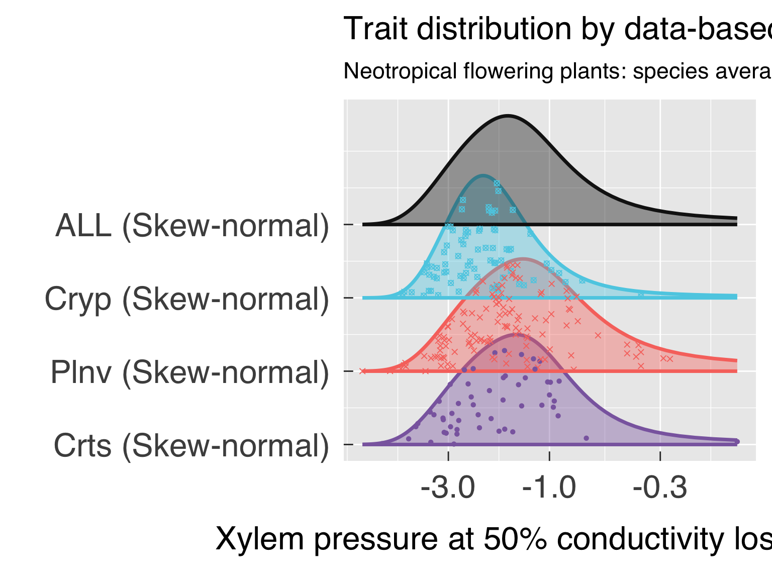
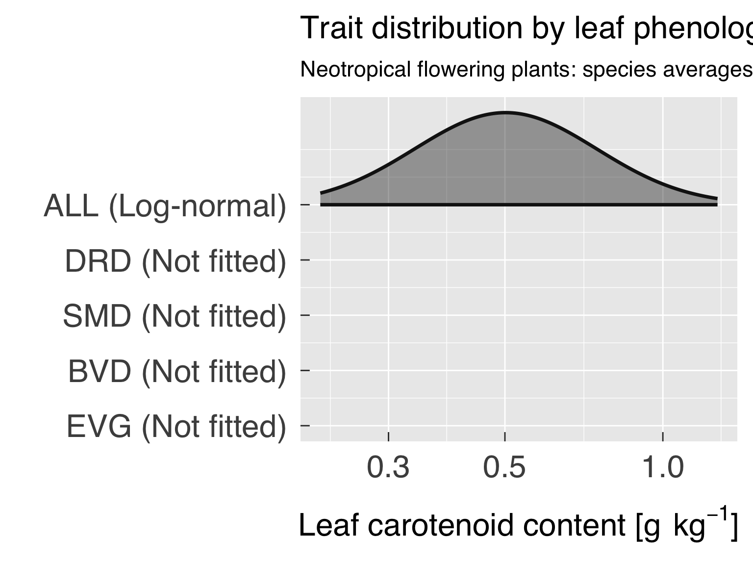
Trait distribution
Here we fit distributions for each trait, separated by the category
that is differentiated by colour. We test multiple distributions and
pick the one that yields the lowest
if (reload_SMA_trait && file.exists(rdata_distr)){
   # Reload data
   cat0(" + Reload trait distributions.")
   dummy = load(rdata_distr)
}else{


   # Load some files which will likely be updated as the code is developed.
   source(file.path(util_path,"FindBestDistr.r"),chdir=TRUE)


   # Find the number of sub-classes to test the model
   CategDistr  = CategExtra %>%
      filter( ( (XYUse %in% "Colour") | (TraitID %in% 0L) ) & (! duplicated(Class))) %>%
      mutate( TraitName = ifelse( test = TraitID %in% 0L, yes = "Cluster", no = try_trait$Name[match(TraitID,try_trait$TraitID)]))
   CntCategDistr = nrow(CategDistr)+1L


   # Select reference data set for trade-off analysis
   DataTRY = switch( EXPR       = fit_taxon
                   , Individual = TidyTRY
                   , Species    = SpeciesTRY
                   , Genus      = GenusTRY
                   , stop("Invalid settings for variable \"fit_taxon\".")
                   )#end switch

   # Find out how many traits we will seek to fit a distribution
   cat0(" + Fit trait distribution")
   xFitDistr = which( (try_trait$Type %in% "numeric") & (! try_trait$Allom))
   CntDistr  = length(xFitDistr)


   # Load settings for the x axis.
   yUniq       = c("ALL"      ,CategDistr$Class  )
   yTraitID    = c(NA_integer_,CategDistr$TraitID)
   yTraitClass = ifelse( test = yTraitID %gt% 0L
                       , yes  = try_trait$Name[match(yTraitID,try_trait$TraitID)]
                       , no   = ifelse(test=yTraitID %eq% 0L,yes="Cluster",no="All")
                       )#end ifelse

   # Save objects for distribution plots:
   # InfoDistr is the tibble with the coefficients and goodness-of-fit metrics
   InfoDistr  = tibble( x          = rep(try_trait$Name[xFitDistr],each=CntCategDistr)
                      , xLwr       = rep(NA_real_                 ,times=CntDistr*CntCategDistr)
                      , xUpr       = rep(NA_real_                 ,times=CntDistr*CntCategDistr)
                      , Class      = rep(yUniq                    ,times=CntDistr)
                      , TraitClass = rep(yTraitClass              ,times=CntDistr)
                      , N          = rep(0L                       ,times=CntDistr*CntCategDistr)
                      , Distrib    = rep(NA_character_            ,times=CntDistr*CntCategDistr)
                      , First      = rep(NA_real_                 ,times=CntDistr*CntCategDistr)
                      , SE_First   = rep(NA_real_                 ,times=CntDistr*CntCategDistr)
                      , Second     = rep(NA_real_                 ,times=CntDistr*CntCategDistr)
                      , SE_Second  = rep(NA_real_                 ,times=CntDistr*CntCategDistr)
                      , Third      = rep(NA_real_                 ,times=CntDistr*CntCategDistr)
                      , SE_Third   = rep(NA_real_                 ,times=CntDistr*CntCategDistr)
                      , Mean       = rep(NA_real_                 ,times=CntDistr*CntCategDistr)
                      , StdDev     = rep(NA_real_                 ,times=CntDistr*CntCategDistr)
                      , Skewness   = rep(NA_real_                 ,times=CntDistr*CntCategDistr)
                      , Kurtosis   = rep(NA_real_                 ,times=CntDistr*CntCategDistr)
                      , Median     = rep(NA_real_                 ,times=CntDistr*CntCategDistr)
                      , LogLik     = rep(NA_real_                 ,times=CntDistr*CntCategDistr)
                      , AIC        = rep(NA_real_                 ,times=CntDistr*CntCategDistr)
                      , BIC        = rep(NA_real_                 ,times=CntDistr*CntCategDistr)
                      )#end tibble

   # Copy fitted model for all
   xGlob             = which(InfoDistr$Class %in% "ALL")
   xCopy             = match(InfoDistr$x,GlobDistr$x)[xGlob]
   InfoDistr[xGlob,] = GlobDistr[xCopy,,drop=FALSE]


   # Skip rows that we have already computed.
   yLoop = which(! (InfoDistr$Class %in% "ALL") )


   # Loop through the variables we will fit distributions
   for (x in seq_along(xFitDistr)){
      # Load settings for the y axis.
      xIndex   = xFitDistr[x]
      xTrait   = try_trait$TraitID[xIndex]
      xName    = try_trait$Name   [xIndex]
      xDesc    = try_trait$Desc   [xIndex]
      xUnit    = try_trait$Unit   [xIndex]
      xTrans   = try_trait$Trans  [xIndex]
      cat0(" + Fit the best distribution model for ",xDesc,".")

      # Select valid points
      xSel = is.finite(DataTRY[[xName]])

      for (y in yLoop){
         # Select category (or everything)
         yName  = InfoDistr$TraitClass[y]
         if (yName %in% "Cluster"){
            yDesc = "Data-based cluster"
         }else{
            yDesc = try_trait$Desc[match(yName,try_trait$Name)]
         }#end if (yName %in% "Cluster")
         yCateg = InfoDistr$Class     [y]
         ySel   = DataTRY[[yName]] %in% yCateg
         cat0("   - ",yDesc," category: ",yCateg,".")

         # Select univariate data
         xySel  = xSel & ySel
         if (sum(xySel) > 0L){
            xData  = DataTRY[[xName]][xSel & ySel]
            suppressWarnings({xDistr = FindBestDistr(x=xData,nx_min=n_fit_min,verbose=FALSE)})

            # Copy summary information to the data table
            xy = which( ( InfoDistr$x        %in% xName  )
                      & ( InfoDistr$Class    %in% yCateg )
            )#end which
            InfoDistr$xLwr     [xy] = xDistr$xLwr
            InfoDistr$xUpr     [xy] = xDistr$xUpr
            InfoDistr$N        [xy] = xDistr$N
            InfoDistr$Distrib  [xy] = xDistr$Distr
            InfoDistr$First    [xy] = xDistr$First
            InfoDistr$SE_First [xy] = xDistr$SE_First
            InfoDistr$Second   [xy] = xDistr$Second
            InfoDistr$SE_Second[xy] = xDistr$SE_Second
            InfoDistr$Third    [xy] = xDistr$Third
            InfoDistr$SE_Third [xy] = xDistr$SE_Third
            InfoDistr$LogLik   [xy] = xDistr$LogLik
            InfoDistr$Mean     [xy] = xDistr$Mean
            InfoDistr$StdDev   [xy] = xDistr$StdDev
            InfoDistr$Skewness [xy] = xDistr$Skewness
            InfoDistr$Kurtosis [xy] = xDistr$Kurtosis
            InfoDistr$Median   [xy] = xDistr$Median
            InfoDistr$BIC      [xy] = xDistr$BIC
         }else{
            cat0("     * Too few valid points (n=",sum(xySel),"). Do not fit distribution.")
         }#end if (sum(xySel) >= n_fit_min)
      }#end for (y in sequence(CntCategDistr))
   }#end for (x in seq_along(xFitDistr))


   # Save SMA models
   cat0(" + Save fitted distributions models to ",basename(rdata_distr))
   dummy = save( list              = c( "InfoDistr" )
               , file              = rdata_distr
               , compress          = "xz"
               , compression_level = 9
               )#end save
}#end if (reload_SMA_trait && file.exists(rdata_distr))

# Write CSV files with trait summaries
cat0(" + Write CSV file with trait distribution information:")
dummy = write_csv( x = InfoDistr, file = distr_summ, na = "")
Trait trade-off relationships for most traits
In this part, we develop standardised major axis fittings between
most traits, using a selected trait as reference.
# Check whether to reload data or fit SMA.
if (reload_SMA_trait && file.exists(rdata_SMA_trait)){
   # Reload data
   cat0(" + Reload trait trade-off relationships.")
   dummy = load(rdata_SMA_trait)
}else{

   # Select reference data set for trade-off analysis
   DataTRY = switch( EXPR       = fit_taxon
                   , Individual = TidyTRY
                   , Species    = SpeciesTRY
                   , Genus      = GenusTRY
                   , stop("Invalid settings for variable \"fit_taxon\".")
                   )#end switch

   # Load settings for the x axis.
   x      = xsma_idx
   xTrait = try_trait$TraitID[x]
   xName  = try_trait$Name   [x]
   xDesc  = try_trait$Desc   [x]
   xUnit  = try_trait$Unit   [x]
   xTrans = try_trait$Trans  [x]

   # Select valid data for the y axis
   xSel = switch( EXPR     = xTrans
                , identity = is.finite(DataTRY[[xName]])
                , log      = DataTRY[[xName]] %gt% 0.
                , neglog   = DataTRY[[xName]] %lt% 0.
                , sqrt     = DataTRY[[xName]] %ge% 0.
                , cbrt     = is.finite(DataTRY[[xName]])
                , stop(paste0(" Invalid transformation for trait ",xName," (TraitID = ",xTrait,")."))
                )#end switch

   # Set forward and backward transformation for x variables
   xForFun  = switch( EXPR     = xTrans
                    , identity = force
                    , log      = log
                    , neglog   = neglog
                    , sqrt     = sqrt
                    , cbrt     = cbrt
                    )#end switch
   xBackFun = switch( EXPR     = xTrans
                    , identity = force
                    , log      = exp
                    , neglog   = negexp
                    , sqrt     = function(x){x^2}
                    , cbrt     = function(x){x^3}
                    )#end switch

   # Define the range for which we will generate a relationship
   xValue  = xForFun(DataTRY[[xName]])
   xRange  = suppressWarnings(range(xValue,finite=TRUE))
   xPred   = seq(from=xRange[1],to=xRange[2],length.out=n_predict)
   xSave   = xBackFun(xPred)
   CntPred = length(xPred)

   # Find out how many SMA fits we will seek
   yFitSMA = which(try_trait$SMA & (! (try_trait$Name %in% xName)))
   CntSMA  = length(yFitSMA)

   # Find the number of sub-classes to test the model
   CategSMA  = CategExtra %>%
      filter( ( (XYUse %in% "Colour") | (TraitID %in% 0L) ) & (! duplicated(Class))) %>%
      mutate( TraitName = ifelse( test = TraitID %in% 0L, yes = "Cluster", no = try_trait$Name[match(TraitID,try_trait$TraitID)]))

   CategALL  = CategExtra[1L,,drop=FALSE] %>%
      mutate( TraitID   = NA_integer_
            , Class     = "ALL"
            , TRYClass  = "All data"
            , Colour    = "#161616"
            , Symbol    = 15L
            , TraitName = "All"
            )#end mutate
   CategUKN  = CategExtra[1L,,drop=FALSE] %>%
      mutate( TraitID   = NA_integer_
            , Class     = "UKN"
            , TRYClass  = "Unknown"
            , Colour    = "#AAAAAA"
            , Symbol    = 0L
            , TraitName = "Unknown"
            )#end mutate
   CategSMA    = rbind(CategSMA,CategUKN,CategALL)
   CntCategSMA = nrow(CategSMA)


   # Save objects for SMA predictions:
   # PredSMA is the tibble that will be saved for plotting (back-transformed)
   # InfoSMA is the tibble with the coefficients and goodness-of-fit metrics
   PredSMA  = tibble( xPred      = rep(xPred,times=CntCategSMA)
                    , x          = rep(xSave,times=CntCategSMA)
                    , Class      = rep(CategSMA$Class,each=CntPred)
                    , TraitClass = rep(CategSMA$TraitName,each=CntPred)
                    )#end tibble
   PredSMA  = PredSMA %>%
      rename_at( vars("x"), ~c(xName))

   InfoSMA  = tibble( x               = rep(xName,times=CntSMA*CntCategSMA)
                    , y               = rep(try_trait$Name[yFitSMA],each=CntCategSMA)
                    , Class           = rep(CategSMA$Class    ,times=CntSMA)
                    , TraitClass      = rep(CategSMA$TraitName,times=CntSMA)
                    , xTrans          = rep(xTrans,times=CntSMA*CntCategSMA)
                    , yTrans          = rep(try_trait$Trans[yFitSMA],each=CntCategSMA)
                    , Intercept       = rep(NA_real_,times=CntSMA*CntCategSMA)
                    , Intercept_LwrCI = rep(NA_real_,times=CntSMA*CntCategSMA)
                    , Intercept_UprCI = rep(NA_real_,times=CntSMA*CntCategSMA)
                    , Slope           = rep(NA_real_,times=CntSMA*CntCategSMA)
                    , Slope_LwrCI     = rep(NA_real_,times=CntSMA*CntCategSMA)
                    , Slope_UprCI     = rep(NA_real_,times=CntSMA*CntCategSMA)
                    , N               = rep(0L      ,times=CntSMA*CntCategSMA)
                    , R2              = rep(NA_real_,times=CntSMA*CntCategSMA)
                    , pValue          = rep(NA_real_,times=CntSMA*CntCategSMA)
                    )#end c

   # Loop through the SMA variables
   for (y in seq_along(yFitSMA)){
      # Load settings for the y axis.
      yIndex   = yFitSMA[y]
      yTrait   = try_trait$TraitID[yIndex]
      yName    = try_trait$Name   [yIndex]
      yDesc    = try_trait$Desc   [yIndex]
      yUnit    = try_trait$Unit   [yIndex]
      yTrans   = try_trait$Trans  [yIndex]
      yNameLwr = paste0(yName,"_Lower")
      yNameUpr = paste0(yName,"_Upper")
      cat0(" + Fit the SMA model for ",yDesc,".")

      # Select valid data for the y axis
      ySel = switch( EXPR     = yTrans
                   , identity = is.finite(DataTRY[[yName]])
                   , log      = DataTRY[[yName]] %gt% 0.
                   , neglog   = DataTRY[[yName]] %lt% 0.
                   , sqrt     = DataTRY[[yName]] %ge% 0.
                   , cbrt     = is.finite(DataTRY[[yName]])
                   , stop(paste0(" Invalid transformation for trait ",yName," (TraitID = ",yTrait,")."))
                   )#end switch

      # Set forward and backward transformation for x variables
      yForFun  = switch( EXPR     = yTrans
                       , identity = force
                       , log      = log
                       , neglog   = neglog
                       , sqrt     = sqrt
                       , cbrt     = cbrt
                       )#end switch
      yBackFun = switch( EXPR     = yTrans
                       , identity = force
                       , log      = exp
                       , neglog   = negexp
                       , sqrt     = function(x){x^2}
                       , cbrt     = function(x){x^3}
                       )#end switch

      # Initialise predicted variable
      PredSMA  = PredSMA %>%
         mutate( y       = rep(NA_real_,nrow(PredSMA))
               , y_Lower = rep(NA_real_,nrow(PredSMA))
               , y_Upper = rep(NA_real_,nrow(PredSMA))
               )#end mutate

      for (z in sequence(CntCategSMA)){
         # Define trait selection
         zTrait = CategSMA$TraitID[z]
         zCateg = CategSMA$Class  [z]
         if (is.na(zTrait)){
            # No selection, use all available data.
            zName = "All"
            zDesc = "All data"
            zSel  = rep(TRUE,nrow(DataTRY))
         }else if(zTrait %in% 0L){
            # Data-based cluster class
            zName  = CategSMA$TraitName[z]
            zDesc  = "Data-based cluster class"
            zSel   = DataTRY[[zName]] %in% zCateg
         }else{
            zIndex = match(zTrait,try_trait$TraitID)
            zName  = try_trait$Name   [zIndex]
            zDesc  = try_trait$Desc   [zIndex]
            zSel   = DataTRY[[zName]] %in% zCateg
         }#end if (is.na(zTrait))
         cat0("   - ",zDesc," category: ",zCateg,".")

         # Subset and transform data prior to fitting the SMA
         DataFit = DataTRY %>%
            filter(xSel & ySel & zSel) %>%
            select_at( vars(c(xName,yName))) %>%
            rename_at( vars(c(xName,yName)), ~ c("x","y")) %>%
            mutate( x  = xForFun(x), y  = yForFun(y) )

         # Find the correlation between variables. This is used to define the expected sign of the
         # relationship, and to determine whether or not fitting a SMA model
         DataCorr = cor(DataFit$x,DataFit$y)

         # Fit the SMA model only when the
         if ( (nrow(DataFit) %gt% n_fit_min ) && (abs(DataCorr) %ge% SMA_AbsCorrMin) ){


            # Fit the full model
            SlopeH0  = (2L*as.integer(DataCorr %ge% 0.)-1L)
            FitSMA   = sma(formula="y~x",data=DataFit,robust=SMA_Robust,method="SMA",slope.test=SlopeH0)
            SummSMA  = FitSMA$groupsummary

            # Copy coefficients to facilitate
            aFit    = coefficients(FitSMA)[1L]
            bFit    = coefficients(FitSMA)[2L]

            # Save the model predictions for the fitted curve.
            pSel            = PredSMA$Class %in% zCateg
            PredSMA$y[pSel] = aFit + bFit * PredSMA$xPred[pSel]
            PredSMA$y[pSel] = aFit + bFit * PredSMA$xPred[pSel]

            # Copy summary information to the data table
            xyz = which( ( InfoSMA$x     %in% xName  )
                       & ( InfoSMA$y     %in% yName  )
                       & ( InfoSMA$Class %in% zCateg )
                       )#end which
            InfoSMA$Intercept      [xyz] = SummSMA$Int
            InfoSMA$Intercept_LwrCI[xyz] = SummSMA$Int_lowCI
            InfoSMA$Intercept_UprCI[xyz] = SummSMA$Int_highCI
            InfoSMA$Slope          [xyz] = SummSMA$Slope
            InfoSMA$Slope_LwrCI    [xyz] = SummSMA$Slope_lowCI
            InfoSMA$Slope_UprCI    [xyz] = SummSMA$Slope_highCI
            InfoSMA$N              [xyz] = SummSMA$n
            InfoSMA$R2             [xyz] = SummSMA$r2
            InfoSMA$pValue         [xyz] = SummSMA$pval

            # Find confidence bands. Sometimes the bootstrap samples may be really off, especially
            # when not fitting a robust model. We check that confidence bands are not outside the
            # expected value. If not, then we keep trying until it works.
            Iterate = TRUE
            Success = FALSE
            it      = 0L
            while (Iterate && (it %lt% SMA_MaxIter)){
               # Update iteration count.
               it = it + 1L
               cat0("     * Find confidence bands. (attempt ",it,").")

               BootSMA  = DataFit %>%
                  modelr::bootstrap(n=n_boot, id = "BootID") %>%
                  group_by(BootID) %>%
                  mutate( .
                        , FitSMA=map(strap, ~ sma(formula="y~x",data=.,method="SMA",robust=SMA_Robust,slope.test=SlopeH0))
                        ) %>% #end mutate
                  ungroup() %>%
                  mutate( .
                        , Intercept = map_dbl(FitSMA, ~coefficients(.)[1L])
                        , Slope     = map_dbl(FitSMA, ~coefficients(.)[2L])
                        ) %>% #end mutate
                  do ( data.frame( yPred = .$Intercept + .$Slope * PredSMA$xPred[pSel]
                                 , xPred = PredSMA$xPred[pSel]                         ) ) %>%
                  ungroup() %>%
                  group_by(.,xPred) %>%
                  summarise( y_Lower = quantile(yPred,probs=SMA_ConfLwr,na.rm=TRUE,names=FALSE)
                           , y_Upper = quantile(yPred,probs=SMA_ConfUpr,na.rm=TRUE,names=FALSE)
                           ) %>% #end summarise
                  ungroup()

               # Copy to the model main structure
               PredSMA$y_Lower[pSel] = BootSMA$y_Lower
               PredSMA$y_Upper[pSel] = BootSMA$y_Upper

               # Sanity check
               MessSMA = PredSMA %>%
                  filter( is.finite(y) & (! y %wr% c(y_Lower,y_Upper)))

               # Check whether or not to iterate
               Success = nrow(MessSMA) %eq% 0L
               Iterate = (! Success) && (it %lt% SMA_MaxIter)
            }#end while (iterate)

            if (nrow(MessSMA) %gt% 0L) stop(paste0("Failed to find reasonable confidence range after ",SMA_MaxIter," attempts!"))

         }else if (abs(DataCorr) %lt% SMA_AbsCorrMin){
            cat0("     * Correlation ",round(DataCorr,2)," is too low to fit a model.")
         }else{
            cat0("     * Not enought points to fit a model.")
         }#end if (nrow(FitSMA) %gt% n_fit_min)

      }#end for (z in sequence(CntCategSMA))


      # Back-transform the fitted curve, and rename variable
      PredSMA = PredSMA %>%
         mutate(y=yBackFun(y), y_Lower = yBackFun(y_Lower), y_Upper = yBackFun(y_Upper)) %>%
         rename_at( vars(c("y","y_Lower","y_Upper")), ~ c(yName,yNameLwr,yNameUpr))

      IsOdd   = ( is.finite(PredSMA[[yName]])
                & (! PredSMA[[yName]] %wr% c(PredSMA[[yNameLwr]],PredSMA[[yNameUpr]]) ) )
      MessSMA = PredSMA %>% filter(IsOdd)
      if (nrow(MessSMA) %gt% 0L) stop("Expected values outside confidence range after back-transformation. Odd!")

      #
   }#end for (y in yloop)


   # Save SMA models
   cat0(" + Save SMA models to ",basename(rdata_SMA_trait))
   dummy = save( list              = c( "DataTRY","PredSMA","InfoSMA", "CategSMA")
               , file              = rdata_SMA_trait
               , compress          = "xz"
               , compression_level = 9
               )#end save
}#end if (reload_SMA_trait && file.exists(rdata_SMA_trait))


# Write CSV files with trait summaries
cat0(" + Write CSV file with SMA information:")
dummy = write_csv( x = InfoSMA, file = SMA_summ, na = "")
Because photosynthetic traits have limited measurements and tend to
be correlated, we fit standardised major axis fittings that are specific
to photosynthetic traits. Similar to the general SMA fitting, we pick
one photosynthesis trait as reference.
# Check whether to reload data or fit SMA.
if (reload_SMA_photo && file.exists(rdata_SMA_photo)){
   # Reload data
   cat0(" + Reload trait trade-off relationships for photosynthetic traits.")
   dummy = load(rdata_SMA_photo)
}else{

   # Select reference data set for trade-off analysis
   DataTRY = switch( EXPR       = fit_taxon
                   , Individual = TidyTRY
                   , Species    = SpeciesTRY
                   , Genus      = GenusTRY
                   , stop("Invalid settings for variable \"fit_taxon\".")
                   )#end switch

   # Load settings for the x axis.
   x      = xphoto_idx
   xTrait = try_trait$TraitID[x]
   xName  = try_trait$Name   [x]
   xDesc  = try_trait$Desc   [x]
   xUnit  = try_trait$Unit   [x]
   xTrans = try_trait$Trans  [x]

   # Select valid data for the y axis
   xSel = switch( EXPR     = xTrans
                , identity = is.finite(DataTRY[[xName]])
                , log      = DataTRY[[xName]] %gt% 0.
                , neglog   = DataTRY[[xName]] %lt% 0.
                , sqrt     = DataTRY[[xName]] %ge% 0.
                , cbrt     = is.finite(DataTRY[[xName]])
                , stop(paste0(" Invalid transformation for trait ",xName," (TraitID = ",xTrait,")."))
                )#end switch

   # Set forward and backward transformation for x variables
   xForFun  = switch( EXPR     = xTrans
                    , identity = force
                    , log      = log
                    , neglog   = neglog
                    , sqrt     = sqrt
                    , cbrt     = cbrt
                    )#end switch
   xBackFun = switch( EXPR     = xTrans
                    , identity = force
                    , log      = exp
                    , neglog   = negexp
                    , sqrt     = function(x){x^2}
                    , cbrt     = function(x){x^3}
                    )#end switch

   # Define the range for which we will generate a relationship
   xValue  = xForFun(DataTRY[[xName]])
   xRange  = suppressWarnings(range(xValue,finite=TRUE))
   xPred   = seq(from=xRange[1],to=xRange[2],length.out=n_predict)
   xSave   = xBackFun(xPred)
   CntPred = length(xPred)

   # Find out how many SMA fits we will seek
   yFitPhoto = which(try_trait$SMA & try_trait$Photo & (! (try_trait$Name %in% xName)))
   CntPhoto  = length(yFitPhoto)

   # Find the number of sub-classes to test the model
   CategPhoto  = CategExtra %>%
      filter( ( (XYUse %in% "Colour") | (TraitID %in% 0L) ) & (! duplicated(Class))) %>%
      mutate( TraitName = ifelse( test = TraitID %in% 0L, yes = "Cluster", no = try_trait$Name[match(TraitID,try_trait$TraitID)]))

   CategALL  = CategExtra[1L,,drop=FALSE] %>%
      mutate( TraitID   = NA_integer_
            , Class     = "ALL"
            , TRYClass  = "All data"
            , Colour    = "#161616"
            , Symbol    = 15L
            , TraitName = "All"
            )#end mutate
   CategUKN  = CategExtra[1L,,drop=FALSE] %>%
      mutate( TraitID   = NA_integer_
            , Class     = "UKN"
            , TRYClass  = "Unknown"
            , Colour    = "#AAAAAA"
            , Symbol    = 0L
            , TraitName = "Unknown"
            )#end mutate
   CategPhoto    = rbind(CategPhoto,CategUKN,CategALL)
   CntCategPhoto = nrow(CategPhoto)


   # Save objects for SMA predictions for photosynthesis parameters:
   # PredPhoto is the tibble that will be saved for plotting (back-transformed)
   # InfoPhoto is the tibble with the coefficients and goodness-of-fit metrics
   PredPhoto  = tibble( xPred      = rep(xPred,times=CntCategSMA)
                      , x          = rep(xSave,times=CntCategSMA)
                      , Class      = rep(CategSMA$Class,each=CntPred)
                      , TraitClass = rep(CategSMA$TraitName,each=CntPred)
                      )#end tibble
   PredPhoto  = PredPhoto %>%
      rename_at( vars("x"), ~c(xName))

   InfoPhoto  = tibble( x               = rep(xName,times=CntPhoto*CntCategPhoto)
                      , y               = rep(try_trait$Name[yFitPhoto],each=CntCategPhoto)
                      , Class           = rep(CategPhoto$Class    ,times=CntPhoto)
                      , TraitClass      = rep(CategPhoto$TraitName,times=CntPhoto)
                      , xTrans          = rep(xTrans,times=CntPhoto*CntCategPhoto)
                      , yTrans          = rep(try_trait$Trans[yFitPhoto],each=CntCategPhoto)
                      , Intercept       = rep(NA_real_,times=CntPhoto*CntCategPhoto)
                      , Intercept_LwrCI = rep(NA_real_,times=CntPhoto*CntCategPhoto)
                      , Intercept_UprCI = rep(NA_real_,times=CntPhoto*CntCategPhoto)
                      , Slope           = rep(NA_real_,times=CntPhoto*CntCategPhoto)
                      , Slope_LwrCI     = rep(NA_real_,times=CntPhoto*CntCategPhoto)
                      , Slope_UprCI     = rep(NA_real_,times=CntPhoto*CntCategPhoto)
                      , N               = rep(0L      ,times=CntPhoto*CntCategPhoto)
                      , R2              = rep(NA_real_,times=CntPhoto*CntCategPhoto)
                      , pValue          = rep(NA_real_,times=CntPhoto*CntCategPhoto)
                      )#end c

   # Loop through the SMA (Photosynthesis) variables
   for (y in seq_along(yFitPhoto)){
      # Load settings for the y axis.
      yIndex   = yFitPhoto[y]
      yTrait   = try_trait$TraitID[yIndex]
      yName    = try_trait$Name   [yIndex]
      yDesc    = try_trait$Desc   [yIndex]
      yUnit    = try_trait$Unit   [yIndex]
      yTrans   = try_trait$Trans  [yIndex]
      yNameLwr = paste0(yName,"_Lower")
      yNameUpr = paste0(yName,"_Upper")
      cat0(" + Fit the SMA (Photosynthesis) model for ",yDesc,".")

      # Select valid data for the y axis
      ySel = switch( EXPR     = yTrans
                   , identity = is.finite(DataTRY[[yName]])
                   , log      = DataTRY[[yName]] %gt% 0.
                   , neglog   = DataTRY[[yName]] %lt% 0.
                   , sqrt     = DataTRY[[yName]] %ge% 0.
                   , cbrt     = is.finite(DataTRY[[yName]])
                   , stop(paste0(" Invalid transformation for trait ",yName," (TraitID = ",yTrait,")."))
                   )#end switch

      # Set forward and backward transformation for x variables
      yForFun  = switch( EXPR     = yTrans
                       , identity = force
                       , log      = log
                       , neglog   = neglog
                       , sqrt     = sqrt
                       , cbrt     = cbrt
                       )#end switch
      yBackFun = switch( EXPR     = yTrans
                       , identity = force
                       , log      = exp
                       , neglog   = negexp
                       , sqrt     = function(x){x^2}
                       , cbrt     = function(x){x^3}
                       )#end switch

      # Initialise predicted variable
      PredPhoto  = PredPhoto %>%
         mutate( y       = rep(NA_real_,nrow(PredPhoto))
               , y_Lower = rep(NA_real_,nrow(PredPhoto))
               , y_Upper = rep(NA_real_,nrow(PredPhoto))
               )#end mutate

      for (z in sequence(CntCategPhoto)){
         # Define trait selection
         zTrait = CategPhoto$TraitID[z]
         zCateg = CategPhoto$Class  [z]
         if (is.na(zTrait)){
            # No selection, use all available data.
            zName = "All"
            zDesc = "All data"
            zSel  = rep(TRUE,nrow(DataTRY))
         }else if(zTrait %in% 0L){
            # Data-based cluster class
            zName  = CategPhoto$TraitName[z]
            zDesc  = "Data-based cluster class"
            zSel   = DataTRY[[zName]] %in% zCateg
         }else{
            zIndex = match(zTrait,try_trait$TraitID)
            zName  = try_trait$Name   [zIndex]
            zDesc  = try_trait$Desc   [zIndex]
            zSel   = DataTRY[[zName]] %in% zCateg
         }#end if (is.na(zTrait))
         cat0("   - ",zDesc," category: ",zCateg,".")

         # Subset and transform data prior to fitting the SMA (Photosynthesis)
         DataFit = DataTRY %>%
            filter(xSel & ySel & zSel) %>%
            select_at( vars(c(xName,yName))) %>%
            rename_at( vars(c(xName,yName)), ~ c("x","y")) %>%
            mutate( x  = xForFun(x), y  = yForFun(y) )

         # Find the correlation between variables. This is used to define the expected sign of the
         # relationship, and to determine whether or not fitting a SMA model (Photosynthesis)
         DataCorr = cor(DataFit$x,DataFit$y)

         # Fit the SMA model (Photosynthesis) only when there are enough data points
         if ( (nrow(DataFit) %gt% n_fit_min ) && (abs(DataCorr) %ge% SMA_AbsCorrMin) ){


            # Fit the full model
            SlopeH0    = (2L*as.integer(DataCorr %ge% 0.)-1L)
            FitPhoto   = sma(formula="y~x",data=DataFit,robust=SMA_Robust,method="SMA",slope.test=SlopeH0)
            SummPhoto  = FitPhoto$groupsummary

            # Copy coefficients to facilitate
            aFit    = coefficients(FitPhoto)[1L]
            bFit    = coefficients(FitPhoto)[2L]

            # Save the model predictions for the fitted curve.
            pSel            = PredPhoto$Class %in% zCateg
            PredPhoto$y[pSel] = aFit + bFit * PredPhoto$xPred[pSel]
            PredPhoto$y[pSel] = aFit + bFit * PredPhoto$xPred[pSel]

            # Copy summary information to the data table
            xyz = which( ( InfoPhoto$x     %in% xName  )
                       & ( InfoPhoto$y     %in% yName  )
                       & ( InfoPhoto$Class %in% zCateg )
                       )#end which
            InfoPhoto$Intercept      [xyz] = SummPhoto$Int
            InfoPhoto$Intercept_LwrCI[xyz] = SummPhoto$Int_lowCI
            InfoPhoto$Intercept_UprCI[xyz] = SummPhoto$Int_highCI
            InfoPhoto$Slope          [xyz] = SummPhoto$Slope
            InfoPhoto$Slope_LwrCI    [xyz] = SummPhoto$Slope_lowCI
            InfoPhoto$Slope_UprCI    [xyz] = SummPhoto$Slope_highCI
            InfoPhoto$N              [xyz] = SummPhoto$n
            InfoPhoto$R2             [xyz] = SummPhoto$r2
            InfoPhoto$pValue         [xyz] = SummPhoto$pval

            # Find confidence bands. Sometimes the bootstrap samples may be really off, especially
            # when not fitting a robust model. We check that confidence bands are not outside the
            # expected value. If not, then we keep trying until it works.
            Iterate = TRUE
            Success = FALSE
            it      = 0L
            while (Iterate && (it %lt% SMA_MaxIter)){
               # Update iteration count.
               it = it + 1L
               cat0("     * Find confidence bands. (attempt ",it,").")

               BootPhoto  = DataFit %>%
                  modelr::bootstrap(n=n_boot, id = "BootID") %>%
                  group_by(BootID) %>%
                  mutate( .
                        , FitPhoto=map(strap, ~ sma(formula="y~x",data=.,method="SMA",robust=SMA_Robust,slope.test=SlopeH0))
                        ) %>% #end mutate
                  ungroup() %>%
                  mutate( .
                        , Intercept = map_dbl(FitPhoto, ~coefficients(.)[1L])
                        , Slope     = map_dbl(FitPhoto, ~coefficients(.)[2L])
                        ) %>% #end mutate
                  do ( data.frame( yPred = .$Intercept + .$Slope * PredPhoto$xPred[pSel]
                                 , xPred = PredPhoto$xPred[pSel]                         ) ) %>%
                  ungroup() %>%
                  group_by(.,xPred) %>%
                  summarise( y_Lower = quantile(yPred,probs=SMA_ConfLwr,na.rm=TRUE,names=FALSE)
                           , y_Upper = quantile(yPred,probs=SMA_ConfUpr,na.rm=TRUE,names=FALSE)
                           ) %>% #end summarise
                  ungroup()

               # Copy to the model main structure
               PredPhoto$y_Lower[pSel] = BootPhoto$y_Lower
               PredPhoto$y_Upper[pSel] = BootPhoto$y_Upper

               # Sanity check
               MessPhoto = PredPhoto %>%
                  filter( is.finite(y) & (! y %wr% c(y_Lower,y_Upper)))

               # Check whether or not to iterate
               Success = nrow(MessPhoto) %eq% 0L
               Iterate = (! Success) && (it %lt% SMA_MaxIter)
            }#end while (iterate)

            if (nrow(MessPhoto) %gt% 0L) stop(paste0("Failed to find reasonable confidence range after ",SMA_MaxIter," attempts!"))

         }else if (abs(DataCorr) %lt% SMA_AbsCorrMin){
            cat0("     * Correlation ",round(DataCorr,2)," is too low to fit a model.")
         }else{
            cat0("     * Not enought points to fit a model.")
         }#end if (nrow(FitPhoto) %gt% n_fit_min)

      }#end for (z in sequence(CntCategPhoto))


      # Back-transform the fitted curve, and rename variable
      PredPhoto = PredPhoto %>%
         mutate(y=yBackFun(y), y_Lower = yBackFun(y_Lower), y_Upper = yBackFun(y_Upper)) %>%
         rename_at( vars(c("y","y_Lower","y_Upper")), ~ c(yName,yNameLwr,yNameUpr))

      IsOdd   = ( is.finite(PredPhoto[[yName]])
                & (! PredPhoto[[yName]] %wr% c(PredPhoto[[yNameLwr]],PredPhoto[[yNameUpr]]) ) )
      MessPhoto = PredPhoto %>% filter(IsOdd)
      if (nrow(MessPhoto) %gt% 0L) stop("Expected values outside confidence range after back-transformation. Odd!")

      #
   }#end for (y in yloop)


   # Save SMA models (photosynthesis)
   cat0(" + Save SMA models (Photosynthesis) to ",basename(rdata_SMA_photo))
   dummy = save( list              = c( "DataTRY","PredPhoto","InfoPhoto", "CategPhoto")
               , file              = rdata_SMA_photo
               , compress          = "xz"
               , compression_level = 9
               )#end save
}#end if (reload_SMA_photo && file.exists(rdata_SMA_photo))


# Write CSV files with trait summaries
cat0(" + Write CSV file with SMA information for photosynthesis traits.")
dummy = write_csv( x = InfoPhoto, file = SMAPhoto_summ, na = "")
In this part, we find rank correlation amongst traits.
# Check whether to reload data or find correlation matrix again.
if (reload_corr_trait && file.exists(rdata_corr_trait)){
   # Reload data
   cat0(" + Reload trait trade-off relationships.")
   dummy = load(rdata_corr_trait)
}else{

   # Select reference data set for trade-off analysis
   DataTRY = switch( EXPR       = fit_taxon
                   , Individual = TidyTRY
                   , Species    = SpeciesTRY
                   , Genus      = GenusTRY
                   , stop("Invalid settings for variable \"fit_taxon\".")
                   )#end switch

   # Find out how many SMA fits we will seek
   xyFindCorr        = which(try_trait$SMA)
   xyCombCorr        = as_tibble(data.frame(t(combn(x=xyFindCorr,m=2))))
   names(xyCombCorr) = c("xIndex","yIndex")
   CntComb           = nrow(xyCombCorr)

   # Find the number of sub-classes to test the model
   CategCorr  = CategExtra %>%
      filter( ( (XYUse %in% "Colour") | (TraitID %in% 0L) ) & (! duplicated(Class))) %>%
      mutate( TraitName = ifelse( test = TraitID %in% 0L, yes = "Cluster", no = try_trait$Name[match(TraitID,try_trait$TraitID)]))

   CategALL  = CategExtra[1L,,drop=FALSE] %>%
      mutate( TraitID   = NA_integer_
            , Class     = "ALL"
            , TRYClass  = "All data"
            , Colour    = "#161616"
            , Symbol    = 15L
            , TraitName = "All"
            )#end mutate
   CategUKN  = CategExtra[1L,,drop=FALSE] %>%
      mutate( TraitID   = NA_integer_
            , Class     = "UKN"
            , TRYClass  = "Unknown"
            , Colour    = "#AAAAAA"
            , Symbol    = 0L
            , TraitName = "Unknown"
            )#end mutate
   CategCorr    = rbind(CategCorr,CategUKN,CategALL)
   CntCategCorr = nrow(CategCorr)


   # Save objects for correlations:
   CorrTRY  = tibble( xName       = rep(try_trait$Name[xyCombCorr$xIndex],times=CntCategCorr)
                    , yName       = rep(try_trait$Name[xyCombCorr$yIndex],times=CntCategCorr)
                    , zName       = rep(CategCorr$TraitName,each=CntComb)
                    , Class       = rep(CategCorr$Class    ,each=CntComb)
                    , Correlation = rep(NA_real_   ,times=CntComb*CntCategCorr)
                    , pValue      = rep(NA_real_   ,times=CntComb*CntCategCorr)
                    , nPairs      = rep(NA_integer_,times=CntComb*CntCategCorr)
                    )#end tibble

   # List trait categories that should be compared.
   zLoop = which(! (CategCorr$Class %in% "UKN"))

   # Loop through trait combinations
   for (xy in sequence(CntComb)){
      # Load traits to be correlated
      xIndex = xyCombCorr$xIndex[xy]
      yIndex = xyCombCorr$yIndex[xy]
      xName  = try_trait$Name[xIndex]
      xDesc  = try_trait$Desc[xIndex]
      yName  = try_trait$Name[yIndex]
      yDesc  = try_trait$Desc[yIndex]
      cat0(" + Find correlation between ",xDesc," and ",yDesc,".")

      # Loop through trait classes (plus the special case of correlating everything)
      for (z in zLoop){
         # Find the trait class
         zName  = CategCorr$TraitName[z]
         zClass = CategCorr$Class    [z]
         if (zName %in% "All"){
            DataCorr = DataTRY                                %>%
               filter_at(vars(c(xName,yName)), ~ ! is.na(.x)) %>%
               select_at(c(xName,yName))
         }else{
            DataCorr = DataTRY                                %>%
               filter_at(vars(c(zName)), ~ .x %in% zClass)    %>%
               filter_at(vars(c(xName,yName)), ~ ! is.na(.x)) %>%
               select_at(c(xName,yName))
         }#end if (zName %in% "All")

         # Select entry from correlation table.
         xyzSel  = which((CorrTRY$xName %in% xName) & (CorrTRY$yName %in% yName) & (CorrTRY$Class %in% zClass))

         # Find the number of points available for correlation
         CntCorr                = nrow(DataCorr)
         CorrTRY$nPairs[xyzSel] = CntCorr


         # Find correlation then save the statistic and the p-value.
         if (CntCorr %gt% n_kendall_min){
            CorrNow                     = Kendall::Kendall( x =DataCorr[[xName]], y = DataCorr[[yName]])
            CorrTRY$Correlation[xyzSel] = CorrNow$tau
            CorrTRY$pValue     [xyzSel] = CorrNow$sl
         }#end if (CntCorr %gt% n_kendall_min)

      }#end for (z in zLoop)
   }#end for (xy in sequence(CntComb))


   # Save SMA models
   cat0(" + Save correlation table to ",basename(rdata_corr_trait))
   dummy = save( list              = c( "CorrTRY")
               , file              = rdata_corr_trait
               , compress          = "xz"
               , compression_level = 9
               )#end save
}#end if (reload_corr_trait && file.exists(rdata_corr_trait))

# Write CSV files with trait summaries
cat0(" + Write CSV file with correlation information:")
CorrShow = CorrTRY %>% filter(pValue %le% pmax_kendall_show)
dummy    = write_csv( x = CorrShow, file = corr_summ, na = "")
Overview plots
Trait abundance maps
First, we plot spatial maps of the trait abundance, using the
prescribed bin size and transformation (because data may be highly
concentrated on a few points, it may be a good idea to apply square root
or logarithmic transformation). These are always done at the individual
level, because they do not depend on matches between traits.
# Make sure the data set has coordinates
Lon = try_ancil$Name[try_ancil$DataID %in% c(60L,4705L,4707L)]
Lat = try_ancil$Name[try_ancil$DataID %in% c(59L,4704L,4706L)]
if (plot_abund_map && all(c(length(Lon),length(Lat)) %eq% 1L)){
   # Plot data. Find grid limits
   TraitLoop = sequence(nrow(try_trait))
   LimitLon  = range(TidyTRY[[Lon]],finite=TRUE)
   LimitLat  = range(TidyTRY[[Lat]],finite=TRUE)
   XYWidth   = min(c(diff(LimitLon),diff(LimitLat))) / n_map_bin

   # Create a dummy tibble with missing values around the edge to fix hexagon size
   LimitWest  = LimitLon[1] - 0.08 * diff (LimitLon)
   LimitEast  = LimitLon[2] + 0.08 * diff (LimitLon)
   LimitSouth = LimitLat[1] - 0.08 * diff (LimitLat)
   LimitNorth = LimitLat[2] + 0.08 * diff (LimitLat)
   EdgeLon    = seq(from=LimitWest ,to=LimitEast ,length.out=n_map_bin)
   EdgeLat    = seq(from=LimitSouth,to=LimitNorth,length.out=n_map_bin)
   EdgeWest   = rep(LimitWest ,times=n_map_bin)
   EdgeEast   = rep(LimitEast ,times=n_map_bin)
   EdgeSouth  = rep(LimitSouth,times=n_map_bin)
   EdgeNorth  = rep(LimitNorth,times=n_map_bin)

   EmptyTemplate = tibble( x = c(EdgeWest,EdgeLon  ,EdgeEast,EdgeLon  )
                         , y = c(EdgeLat ,EdgeNorth,EdgeLat ,EdgeSouth)
                         , z = NA_character_
                         )#end tibble
}else{
   TraitLoop = sequence(0L)
}#end if (all(c(length(Lon),length(Lat))) %gt% 0L)

# Loop through traits with potential geo-referenced data
gg_map = list()
for (tr in TraitLoop){
   # Select trait
   TraitName  = try_trait$Name [tr]
   TraitDesc  = try_trait$Desc [tr]
   TraitUnit  = try_trait$Unit [tr]
   TraitType  = try_trait$Type [tr]


   # Exclude rows that are not georeferenced or do not have valid data for the current trait,
   # and check if there are enough points for drawing the map.
   AbundTRY   = TidyTRY %>%
      select_at(vars(c(Lon,Lat,TraitName))) %>%
      filter_at(vars(c(Lon,Lat,TraitName)), all_vars(! is.na(.)))
   CntTrait  = nrow(AbundTRY)
   TraitPlot = CntTrait %ge% n_map_min


   # Plot the map if there are enough points
   if (TraitPlot){
      # Make empty template compatible with the current data
      Empty = EmptyTemplate %>%
         mutate(z = as(z,TraitType)) %>%
         rename_at(vars(x,y,z), ~c(Lon,Lat,TraitName))

      # Append empty template to data so hexagons look all the same.
      AbundTRY = bind_rows(AbundTRY,Empty)

      cat0(" + Plot abundance maps of ",TraitDesc," (",TraitName,").")
      gg_now = ggplot()
      gg_now = gg_now + geom_sf(data=br_states,fill="transparent",colour="grey20",linetype="dashed",size=.15,show.legend=FALSE)
      gg_now = gg_now + geom_sf(data=all_countries,fill="transparent",colour="black",linetype="solid",size=.30,show.legend=FALSE)
      gg_now = gg_now + coord_sf(xlim=LimitLon,ylim=LimitLat)
      gg_now = gg_now + geom_bin_2d(data=AbundTRY,aes_string(x=Lon,y=Lat),binwidth=c(XYWidth,XYWidth))
      gg_now = gg_now + scale_fill_continuous(type = map_colour,direction=-1,trans=map_trans,limits=map_range,oob=squish)

      # Add annotation
      gg_now = gg_now + labs ( x        = element_blank()
                             , y        = element_blank()
                             , title    = TraitDesc
                             , subtitle = paste0("Observation abundance (n=",CntTrait,")")
                             )#end labs

      # Axis theme settings
      gg_now = gg_now + theme_grey( base_size      = gg_ptsz
                                  , base_family    = "Helvetica"
                                  , base_line_size = 0.5
                                  , base_rect_size = 0.5
                                  )#end theme_grey
      gg_now = gg_now + theme( axis.text.x       = element_text( size   = gg_ptsz*0.8
                                                               , margin = unit(rep(0.35,times=4),"char")
                                                               )#end element_text
                             , axis.text.y       = element_text( size   = gg_ptsz*0.8
                                                               , margin = unit(rep(0.35,times=4),"char")
                                                               )#end element_text
                             , axis.ticks.length = unit(-0.2,"char")
                             , axis.title.y      = element_text( size = gg_ptsz * 0.6)
                             , legend.title      = element_text( size = gg_ptsz * 0.6)
                             , plot.margin       = unit(c(0,0,0,0), "mm")
                             )#end theme

      #Stash map
      gg_map[[TraitName]] = gg_now

      #Save map to file
      DeviceLoop = sequence(ndevice)
      for (d in DeviceLoop){
         h_output = paste0("AbundMap-",TraitName,"-",base_suffix,".",gg_device[d])
         dummy    = ggsave( filename = h_output
                          , plot     = gg_now
                          , device   = gg_device[d]
                          , path     = abund_path
                          , units    = gg_units
                          , dpi      = gg_depth
                          , width    = gg_width
                          , height   = gg_height
                          )#end ggsave
      }#end for (d in device_loop)
   }#end if (TraitPlot)

}#end for (tr in TraitLoop)

# If sought, plot images on screen
cnt_gg_map = length(gg_map)
if (gg_screen && (cnt_gg_map %gt% 0L)){
   gg_show = sort(sample.int(n=cnt_gg_map,size=min(cnt_gg_map,3L),replace=FALSE))
   gg_map[gg_show]
}#end if (gg_screen && (length(gg_map) %gt% 0L))
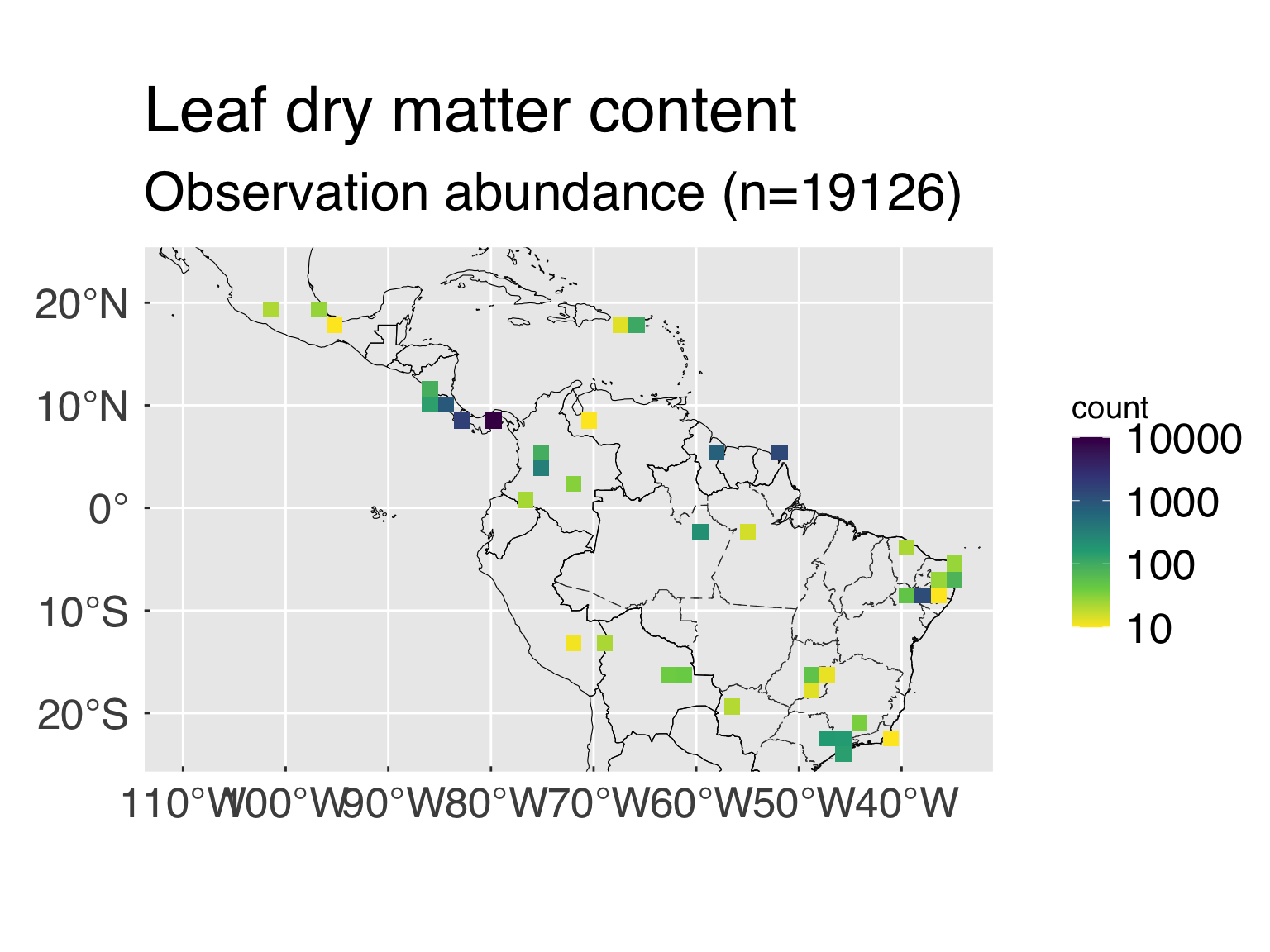
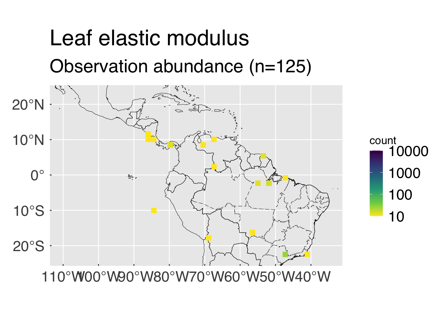

Violin plots
Here we plot violin diagrams segregated by multiple categorical
variables.
# Select reference data set for trade-off analysis
DataTRY = switch( EXPR       = fit_taxon
                , Individual = TidyTRY
                , Species    = SpeciesTRY
                , Genus      = GenusTRY
                , stop("Invalid settings for variable \"fit_taxon\".")
                )#end switch

# Select categories we are interested in plotting.
CategTraitID    = sort(unique(CategExtra$TraitID))
CategTraitID    = CategTraitID[CategTraitID %in% c(0L,try_trait$TraitID)]
CntCategList    = length(CategTraitID)

# Loop through categorical traits and assign all individuals from the same species to the commonest class
gg_violin = list()
CategLoop = if(plot_violin){sequence(CntCategList)}else{sequence(0L)}
#  Loop through the categories
for (w in CategLoop){

   # Select categorical trait
   CategIDNow = CategTraitID[w]
   if (CategIDNow %in% 0L){
      # Handy aliases
      CategName = "Cluster"
      CategDesc = "Trait-based clusters"
   }else{
      # Find settings from try_trait
      z          = match(CategIDNow,try_trait$TraitID)
      if (! is.finite(z)) stop(paste0(" Unrecognised categorical trait ID: ",CategIDNow,"."))

      # Handy aliases
      CategName = try_trait$Name[z]
      CategDesc = try_trait$Desc[z]
   }#end if (CategIDNow %in% 0L)
   cat0(" + Plot violin diagrams grouped by ",CategDesc," (",CategName,").")

   # Select only the lines that are associated with this trait AND are not duplicated.
   InfoNow = CategExtra               %>%
      filter(TraitID %in% CategIDNow) %>%
      filter(! duplicated(Class))
   CntInfoNow = nrow(InfoNow)

   # Filter input data to exclude missing categories
   ViolinTRY = DataTRY %>%
      filter_at(vars(CategName), ~ ! is.na(.x)) %>%
      mutate_at(vars(CategName), ~ factor(.x,levels=InfoNow$Class))

   # Make sure there is anything to plot
   IsPlot = which((try_trait$Type %in% "numeric") & (! try_trait$Allom) & (try_trait$Name %in% names(ViolinTRY)))

   # Loop through all traits, and compare evergreens with drought deciduous.
   for (tr in IsPlot){
      # Select trait
      TraitName  = try_trait$Name [tr]
      TraitDesc  = try_trait$Desc [tr]
      TraitUnit  = try_trait$Unit [tr]
      TraitTrans = try_trait$Trans[tr]
      TraitTrans = switch( EXPR     = try_trait$Trans[tr]
                         , log      = "log10"
                         , neglog   = "neglog10"
                         , try_trait$Trans[tr]
                         )#end switch

      # Ensure that trait is numeric and has valid values for at least 2 categories.
      TraitRange = ViolinTRY %>%
         group_by_at(vars(CategName)) %>%
         summarise_at(vars(TraitName), ~ range(.x,finite=TRUE)) %>%
         ungroup()
      TraitFine  = ViolinTRY %>%
         group_by_at(vars(CategName)) %>%
         summarise_at(vars(TraitName), ~ sum(is.finite(.x)) %ge% n_violin_min) %>%
         ungroup()
      TraitPlot   = sum(TraitFine[[TraitName]]) %ge% 2L

      # Exclude data from categories with too few data points
      CategIgnore  = as.integer(TraitFine[[CategName]])[! TraitFine[[TraitName]]]
      Discard      = as.integer(ViolinTRY[[CategName]]) %in% CategIgnore
      ViolinTRY[[TraitName]][Discard] = NA_real_

      # We only plot this if this trait has anything to be plotted.
      if (TraitPlot){
         # Run Tukey's HSD test for phenological groups
         TraitFormula = as.formula(paste0(TraitName," ~ ",CategName))
         TraitAOV     = aov(TraitFormula,data=ViolinTRY)
         TraitGroup   = HSD.test(TraitAOV,trt=CategName,group=TRUE)$groups
         TraitOrder   = InfoNow$Class[InfoNow$Class %in% rownames(TraitGroup)]
         TraitGroup   = TraitGroup[TraitOrder,,drop=FALSE]

         # Set y axis range, apply an offset for Tukey's HSD tests
         TraitYLim   = range(TraitRange[[TraitName]],finite=TRUE)
         TraitYLwr   = TraitYLim[1L]
         TraitYUpr   = TraitYLim[2L]
         if (TraitTrans %in% "identity"){
            TraitYOff = 0.1 * (TraitYUpr - TraitYLwr)
            TraitYUpr = TraitYUpr + TraitYOff
         }else if (TraitTrans %in% "log10"){
            TraitYLwr = log10(TraitYLwr)
            TraitYUpr = log10(TraitYUpr)
            TraitYOff = 0.1 * (TraitYUpr - TraitYLwr)
            TraitYLwr = 10^TraitYLwr
            TraitYUpr = 10^(TraitYUpr+TraitYOff)
         }else if (TraitTrans %in% "neglog"){
            TraitYLwr = -log10(-TraitYLwr)
            TraitYUpr = -log10(-TraitYUpr)
            TraitYOff =  0.1 * (TraitYUpr - TraitYLwr)
            TraitYLwr = -10^(-TraitYLwr)
            TraitYUpr = -10^(-TraitYUpr-TraitYOff)
         }else if (TraitTrans %in% "sqrt"){
            TraitYLwr = sqrt(TraitYLwr)
            TraitYUpr = sqrt(TraitYUpr)
            TraitYOff = 0.1 * (TraitYUpr - TraitYLwr)
            TraitYLwr = TraitYLwr^2
            TraitYUpr = (TraitYUpr+TraitYOff)^2
         }else if (TraitTrans %in% "cbrt"){
            TraitYLwr = cbrt(TraitYLwr)
            TraitYUpr = cbrt(TraitYUpr)
            TraitYOff = 0.1 * (TraitYUpr - TraitYLwr)
            TraitYLwr = TraitYLwr^3
            TraitYUpr = (TraitYUpr+TraitYOff)^3
         }#end if (TraitTrans %in% "identity")
         TraitYLim   = c(TraitYLwr,TraitYUpr)
         TraitTukey  = tibble( x      = match(rownames(TraitGroup),InfoNow$Class)
                             , y      = rep(x=TraitYUpr,times=nrow(TraitGroup))
                             , labels = TraitGroup$groups
                             )#end tibble

         # Create named vector for phenology classes: this is needed to ensure colours are consistent.
         ViolinLabel  = InfoNow$Class ; names(ViolinLabel ) = InfoNow$Class
         ViolinColour = InfoNow$Colour; names(ViolinColour) = InfoNow$Class

         # Add violins
         gg_now = ggplot(data=ViolinTRY,aes_string(x=CategName,y=TraitName,fill=CategName))
         gg_now = gg_now + scale_x_discrete(labels=ViolinLabel)
         gg_now = gg_now + scale_y_continuous(limits=TraitYLim,trans=TraitTrans)
         gg_now = gg_now + geom_violin(trim=TRUE,show.legend = FALSE,kernel="optcosine",n=2048L)
         gg_now = gg_now + scale_fill_manual(values=ViolinColour)
         gg_now = gg_now + geom_boxplot(width=0.05,fill="grey23",colour="white",outlier.shape=NA,show.legend = FALSE)
         gg_now = gg_now + geom_text( data        = TraitTukey
                                    , mapping     = aes(x=x,y=y,label=labels)
                                    , hjust       = 0.5
                                    , vjust       = 1
                                    , family      = "Helvetica"
                                    , size        = 0.5 * gg_ptsz
                                    , inherit.aes = FALSE
                                    )#end geom_text
         gg_now = gg_now + ggtitle(TraitDesc)
         gg_now = gg_now + xlab(element_blank())
         gg_now = gg_now + ylab(desc.unit(desc=NULL,unit=untab[[TraitUnit]],twolines=FALSE))
         gg_now = gg_now + theme_grey( base_size = gg_ptsz, base_family = "Helvetica",base_line_size = 0.5,base_rect_size =0.5)
         gg_now = gg_now + theme( axis.text.x = element_text( size   = gg_ptsz
                                                            , margin = unit(rep(0.10,times=4),"cm")
                                                            , angle  = 30
                                                            , hjust  = 1
                                                            , vjust  = 1
                                                            )#end element_text
                                , axis.text.y       = element_text( size   = gg_ptsz
                                                                  , margin = unit(rep(0.35,times=4),"cm")
                                                                  )#end element_text
                                , axis.title.y      = element_text( size = gg_ptsz)
                                , plot.title        = element_text( size = gg_ptsz)
                                , axis.ticks.length = unit(-0.25,"cm")
                                )#end theme

         # Save plots.
         DeviceLoop = sequence(ndevice)
         for (d in DeviceLoop){
            h_output = paste0("Violin-",CategName,"-",TraitName,"-",base_suffix,".",gg_device[d])
            dummy    = ggsave( filename = h_output
                             , plot     = gg_now
                             , device   = gg_device[d]
                             , path     = violin_path
                             , units    = gg_units
                             , dpi      = gg_square
                             , width    = gg_square
                             , height   = gg_height
                             )#end ggsave
         }#end for (d in device_loop)

         # Copy gg information to the list
         gg_name = paste0(CategName,"_",TraitName)
         gg_violin[[gg_name]] = gg_now
      }#end if (t_plot)
   }#end for (tr in sequence(n_trait))
}# for (z in sequence(CntCategList))

# If sought, plot images on screen
cnt_gg_violin = length(gg_violin)
if (gg_screen && (cnt_gg_violin %gt% 0L)){
   gg_show = sort(sample.int(n=cnt_gg_violin,size=min(cnt_gg_violin,3L),replace=FALSE))
   gg_violin[gg_show]
}#end if (gg_screen && (length(gg_violin) %gt% 0L))
Gap statistics and silhouette plots
Here we plot the gap statistics and silhouette plots, which are
helpful for defining the ideal number of clusters.
if (plot_stat_cluster){
   cat0(" + Plot optimal cluster analysis diagrams.")

   # Initialise list with GGPlots
   gg_see = list()

   # Create metrics for error plots
   InfoPlot = ClusterInfo %>%
      mutate( gap_lwr = gap - gapSE
            , gap_upr = gap + gapSE
            )#end mutate

   # Retrieve the optimal number of clusters for each method.
   k_opt_sil = length(ClusterOpt$sil$medoids)
   k_opt_gap = length(ClusterOpt$gap$medoids)

   InfoSil = InfoPlot        %>%
      filter(k==k_opt_sil)   %>%
      mutate(Label=paste0("k[O*p*t]==",k_opt_sil))
   InfoGap = InfoPlot        %>%
      filter(k==k_opt_gap)   %>%
      mutate(Label=paste0("k[O*p*t]==",k_opt_gap))

   # First, we plot the silhouette score
   cat0("   - Silhouette score.")
   gg_sil = ggplot(data=InfoPlot,aes(x=k,y=sil_width))
   gg_sil = gg_sil + geom_line(colour="#3A6FB0",size=1.2)
   gg_sil = gg_sil + geom_point(shape=16L,colour="#3A6FB0",size=2.0)
   gg_sil = gg_sil + geom_point( data        = InfoSil
                               , mapping     = aes(x=k,y=sil_width)
                               , shape       = 15L
                               , colour      = "#C53F2D"
                               , size        = 3.0
                               , inherit.aes = FALSE
                               )#end geom_point
   gg_sil = gg_sil + geom_text( data        = InfoSil
                              , mapping     = aes(x=k,y=sil_width,label=Label)
                              , colour      = "#C53F2D"
                              , hjust       = -0.1
                              , vjust       =  1.1
                              , family      = "Helvetica"
                              , parse       = TRUE
                              , size        = 0.25 * gg_ptsz
                              , inherit.aes = FALSE
                              )#end geom_text
   gg_sil = gg_sil + labs( title    = "Silhouette analysis"
                         , subtitle = "Optimal number (red) is the maximum score"
                         , x        = "Number of clusters"
                         , y        = "Silhouette score"
                         )#end labs
   gg_sil = gg_sil + theme_grey( base_size = gg_ptsz, base_family = "Helvetica",base_line_size = 0.5,base_rect_size =0.5)
   gg_sil = gg_sil + theme( axis.text.x = element_text( size   = gg_ptsz
                                                      , margin = unit(rep(0.35,times=4),"cm")
                                                      )#end element_text
                          , axis.text.y       = element_text( size   = gg_ptsz
                                                            , margin = unit(rep(0.35,times=4),"cm")
                                                            )#end element_text
                          , axis.title.y      = element_text( size = gg_ptsz)
                          , plot.title        = element_text( size = gg_ptsz)
                          , plot.subtitle     = element_text( size = 0.7*gg_ptsz)
                          , axis.ticks.length = unit(-0.25,"cm")
                          )#end theme

   # Copy the plot to the list
   gg_see$sil = gg_sil

   # Save plot in every format requested.
   for (d in sequence(ndevice)){
      f_output = paste0("Silhouette_",base_suffix,".",gg_device[d])
      dummy    = ggsave( filename = f_output
                       , plot     = gg_sil
                       , device   = gg_device[d]
                       , path     = trpca_path
                       , width    = gg_width
                       , height   = gg_height
                       , units    = gg_units
                       , dpi      = gg_depth
                       )#end ggsave
   }#end for (o in sequence(nout))


   # First, we plot the gap statistics
   cat0("   - Gap statistics.")
   gg_gap = ggplot(data=InfoPlot,aes(x=k,y=gap,ymin=gap_lwr,ymax=gap_upr))
   gg_gap = gg_gap + geom_line(colour="#3A6FB0",size=0.75)
   gg_gap = gg_gap + geom_point(shape=16L,colour="#3A6FB0",size=2.0)
   gg_gap = gg_gap + geom_errorbar(colour="#3A6FB0",linewidth=0.75,width=1./6.)
   gg_gap = gg_gap + geom_point( data        = InfoGap
                               , mapping     = aes(x=k,y=gap)
                               , shape       = 15L
                               , colour      = "#C53F2D"
                               , size        = 3.0
                               , inherit.aes = FALSE
                               )#end geom_point
   gg_gap = gg_gap + geom_errorbar( data        = InfoGap
                                  , mapping     = aes(x=k,ymin=gap_lwr,ymax=gap_upr)
                                  , colour      = "#C53F2D"
                                  , linewidth   = 0.75
                                  , width       = 1./6.
                                  , inherit.aes = FALSE
                                  )#end geom_point
   gg_gap = gg_gap + geom_text( data        = InfoGap
                              , mapping     = aes(x=k,y=gap,label=Label)
                              , colour      = "#C53F2D"
                              , hjust       = -0.1
                              , vjust       = -0.1
                              , family      = "Helvetica"
                              , parse       = TRUE
                              , size        = 0.25 * gg_ptsz
                              , inherit.aes = FALSE
                              )#end geom_text
   gg_gap = gg_gap + labs( title    = "Gap analysis"
                         , subtitle = "Optimal number (red) based on first maximum above SE"
                         , x        = "Number of clusters"
                         , y        = "Gap Statistic"
                         )#end labs
   gg_gap = gg_gap + theme_grey( base_size = gg_ptsz, base_family = "Helvetica",base_line_size = 0.5,base_rect_size =0.5)
   gg_gap = gg_gap + theme( axis.text.x = element_text( size   = gg_ptsz
                                                      , margin = unit(rep(0.35,times=4),"cm")
                                                      )#end element_text
                          , axis.text.y       = element_text( size   = gg_ptsz
                                                            , margin = unit(rep(0.35,times=4),"cm")
                                                            )#end element_text
                          , axis.title.y      = element_text( size = gg_ptsz)
                          , plot.title        = element_text( size = gg_ptsz)
                          , plot.subtitle     = element_text( size = 0.7*gg_ptsz)
                          , axis.ticks.length = unit(-0.25,"cm")
                          )#end theme

   # Copy the plot to the list
   gg_see$gap = gg_gap

   # Save plot in every format requested.
   for (d in sequence(ndevice)){
      f_output = paste0("GapStatistic",base_suffix,".",gg_device[d])
      dummy    = ggsave( filename = f_output
                       , plot     = gg_gap
                       , device   = gg_device[d]
                       , path     = trpca_path
                       , width    = gg_square
                       , height   = gg_square
                       , units    = gg_units
                       , dpi      = gg_depth
                       )#end ggsave
   }#end for (o in sequence(nout))

   if (gg_screen) gg_see

}#end if (plot_stat_cluster)
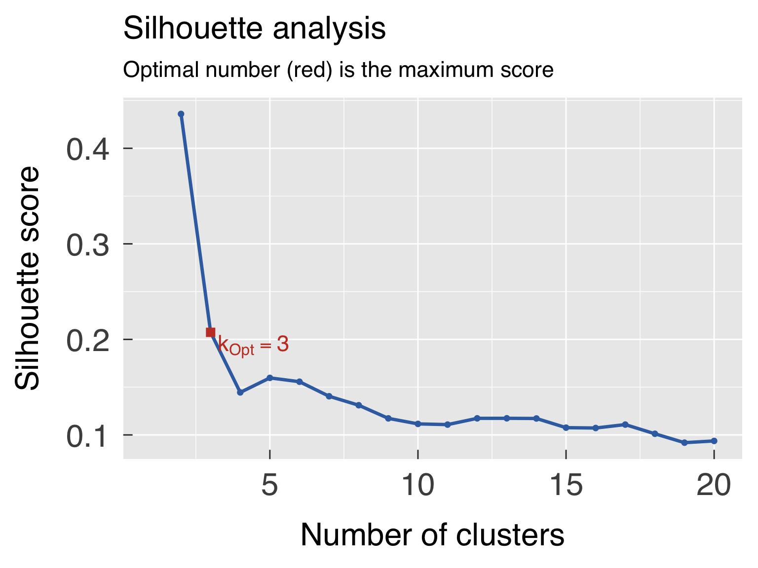
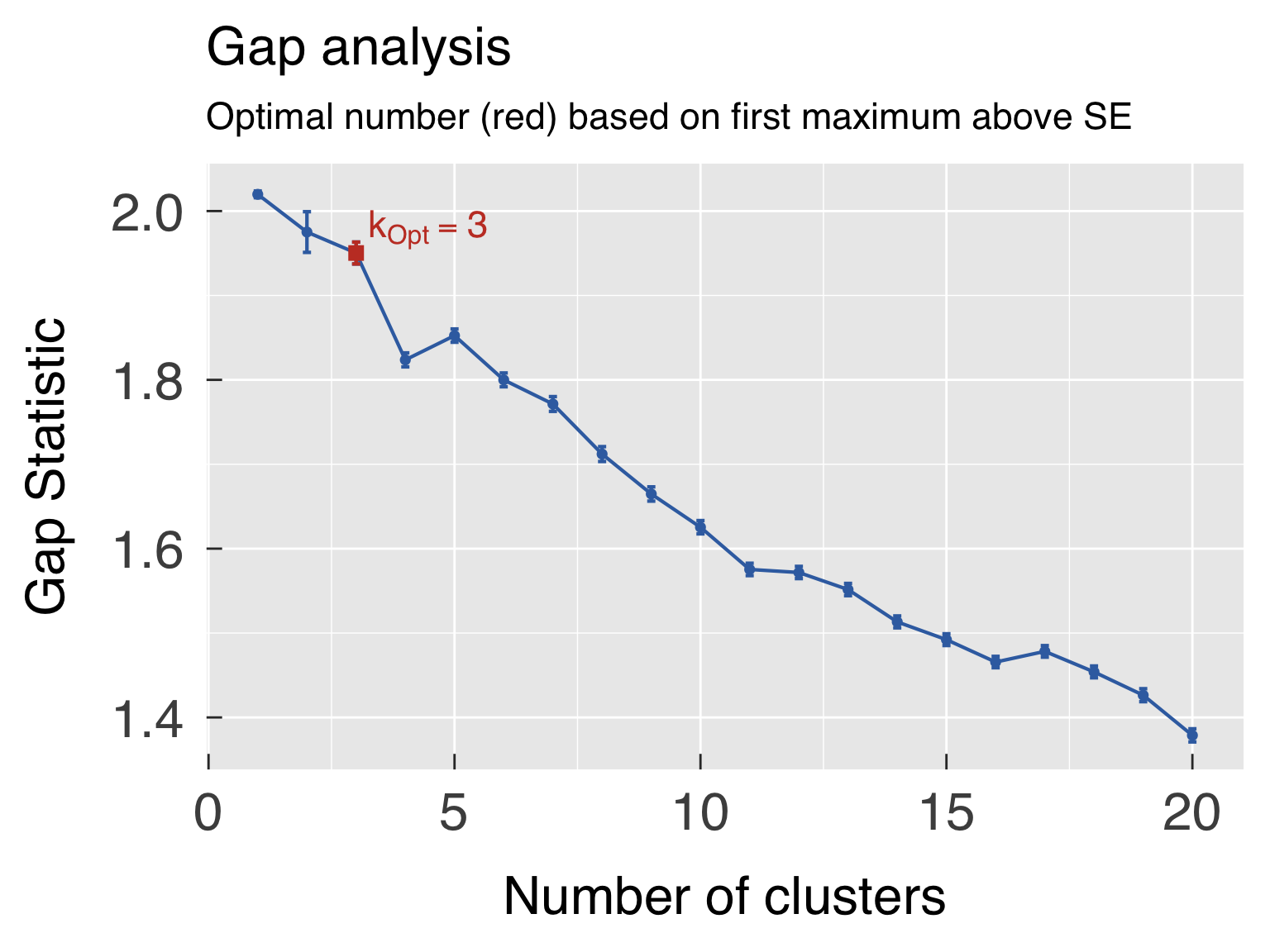
Weighting factors for cluster analysis
Here we plot the gap statistics and silhouette plots, which are
helpful for defining the ideal number of clusters.
if (plot_wgt_cluster){
   cat0(" + Plot weighting factors for cluster analysis.")

   # Arrange data set for showing weights
   WeightTRY = DataInfo %>%
      arrange(Weight) %>%
      mutate( TraitID = try_trait$TraitID[match(Name,try_trait$Name)]
            , Desc    = try_trait$Desc[match(Name,try_trait$Name)]
            , Desc    = ifelse(test = Name %in% "ScientificName"  ,yes="Species",no=Desc)
            , Desc    = ifelse(test = Name %in% "Genus"           ,yes="Genus",no=Desc)
            , Desc    = ifelse(test = Name %in% "Family"          ,yes="Family",no=Desc)
            , Desc    = ifelse(test = Name %in% "Order"           ,yes="Order (Taxonomy)" ,no=Desc)
            , Desc    = ifelse(test = Name %in% "Class"           ,yes="Class (Taxonomy)" ,no=Desc)
            , Desc    = ifelse(test = Name %in% "Phylum"          ,yes="Phylum" ,no=Desc)
            , Desc    = factor(Desc,levels=Desc)
            , Type    = ifelse(test = Type %in% c("factor"   ), yes = "categorical", no = Type)
            , Type    = ifelse(test = Type %in% c("character"), yes = "categorical", no = Type)
            , Type    = ifelse(test = Type %in% c("integer"  ), yes = "ordered"    , no = Type)
            , Type    = str_to_sentence(Type)
            , Type    = factor(Type,levels=sort(unique(Type))))

   CntTypes = nlevels(WeightTRY$Type)
   colTypes = RColorBrewer::brewer.pal(n=max(3L,CntTypes),name="Paired")[sequence(CntTypes)]
   names(colTypes) = levels(WeightTRY$Type)


   # First, we plot the gap statistics
   gg_wgt = ggplot(data=WeightTRY,aes(x=Weight,y=Desc,colour=Type,fill=Type))
   gg_wgt = gg_wgt + geom_col(width=0.8)
   gg_wgt = gg_wgt + scale_fill_manual(values=colTypes)
   gg_wgt = gg_wgt + scale_colour_manual(values=colTypes)
   gg_wgt = gg_wgt + labs( title    = "Dissimilarity matrix weights"
                         , subtitle = "Weigths relative to maximum"
                         , x        = element_blank()
                         , y        = element_blank()
                         )#end labs
   gg_wgt = gg_wgt + theme_grey( base_size = gg_ptsz, base_family = "Helvetica",base_line_size = 0.5,base_rect_size =0.5)
   gg_wgt = gg_wgt + theme( axis.text.x = element_text( size   = gg_ptsz
                                                      , margin = unit(rep(0.35,times=4),"cm")
                                                      )#end element_text
                          , axis.text.y       = element_text( size   = 0.7*gg_ptsz
                                                            , margin = unit(rep(0.35,times=4),"cm")
                                                            )#end element_text
                          , axis.title.y      = element_text( size = 0.8*gg_ptsz)
                          , plot.title        = element_text( size = 0.8*gg_ptsz)
                          , plot.subtitle     = element_text( size = 0.6*gg_ptsz)
                          , axis.ticks.length = unit(-0.25,"cm")
                          , legend.position   = "bottom"
                          , legend.direction  = "horizontal"
                          )#end theme

   # Save plot in every format requested.
   for (d in sequence(ndevice)){
      f_output = paste0("WeightCluster",base_suffix,".",gg_device[d])
      dummy    = ggsave( filename = f_output
                       , plot     = gg_wgt
                       , device   = gg_device[d]
                       , path     = trpca_path
                       , width    = gg_square
                       , height   = gg_square
                       , units    = gg_units
                       , dpi      = gg_depth
                       )#end ggsave
   }#end for (o in sequence(nout))

   if (gg_screen) gg_wgt
}#end if (plot_wgt_cluster)
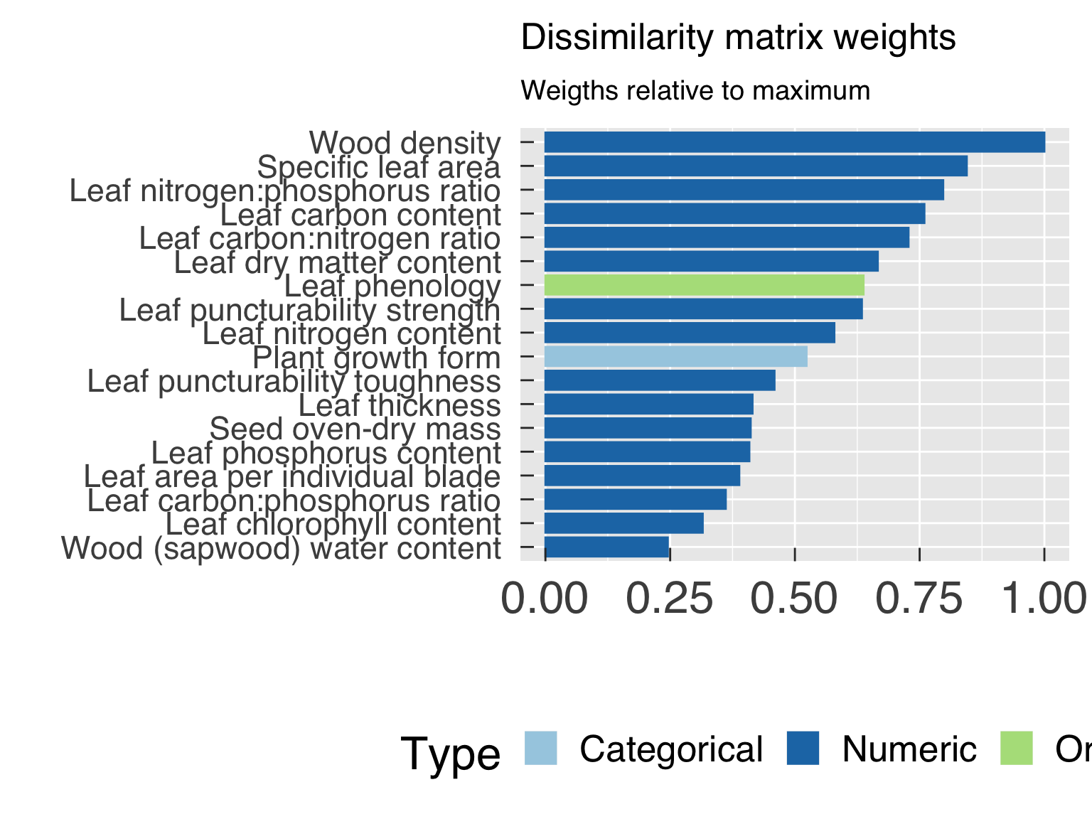
Principal component analysis with numeric traits
Here we run a principal component analysis (PCA) with the traits that
are numeric. PCA requires complete data sets, so we must run an
imputation approach first. Mind that imputation works best when only a
small fraction of the data points is missing. It is very unlikely that
this assumption will hold valid at regional or global scale in the
tropics.
cat0(" + Run the principal component analysis.")
selTrait  = (try_trait$Type %in% "numeric") & try_trait$Cluster & (try_trait$Name %in% names(ClusterTRY))
TraitUse  = names(ClusterTRY)[names(ClusterTRY)   %in% try_trait$Name[selTrait]]
TraitSkip = names(ClusterTRY)[! names(ClusterTRY) %in% TraitUse]
WhichUse  = match(TraitUse,try_trait$Name)
DataUse   = ClusterTRY %>% select_at(all_of(TraitUse ))
DataSkip  = ClusterTRY %>% select_at(all_of(TraitSkip))


# Find the number of sub-classes to test the model
CategPCA  = CategInfo %>%
   filter((XYUse %in% "Colour") & (! duplicated(Class)))
CntCategPCA = nrow(CategPCA)+1L

# Transform variables ahead of the PCA
cat0("   - Transform variables prior to running the PCA.")
for (v in WhichUse){
   # Handy aliases
   vName   = try_trait$Name      [v]
   vDesc   = try_trait$Desc      [v]
   z       = which(GlobDistr$x %in% vName)
   zDistr  = GlobDistr$Distrib[z]
   zFirst  = GlobDistr$First  [z]
   zSecond = GlobDistr$Second [z]
   zThird  = GlobDistr$Third  [z]

   # Pick cumulative distribution function according to the distribution.
   zFun = switch( zDistr
                , "uniform"       = punif
                , "normal"        = pnorm
                , "logistic"      = plogis
                , "skew-normal"   = sn::psn
                , "log-normal"    = plnorm
                , "neglog-normal" = pnlnorm
                , "weibull"       = pweibull
                , "gamma"         = pgamma
                , NA_character_
                )#end switch
   # Decide whether the distribution needs two or three parameters
   if (zDistr %in% "skew-normal"){
      p_vName = zFun(ClusterTRY[[vName]],zFirst,zSecond,zThird)
   }else if (! is.na(zDistr)){
      p_vName = zFun(ClusterTRY[[vName]],zFirst,zSecond)
   }#end if (zDistr %in% "skew-normal")

   # Find the normal distribution equivalent of the value
   DataUse[[vName]] = qnorm(p=p_vName,mean=0.,sd=1.)
   DataUse[[vName]] = ifelse( test = is.finite(DataUse[[vName]])
                            , yes  = DataUse[[vName]]
                            , no   = NA_real_
                            )#end ifelse
}#end for  (z in WhichUse)

# Select data with a sufficient number of data sets
SampUse = DataUse %>%
   summarise(across(everything(), ~ sum(is.finite(.x))))
SdevUse = DataUse %>%
   summarise(across(everything(), ~ sd(.x,na.rm=TRUE)))
SampUse = names(SampUse)[SampUse %ge% n_pca_min]
SdevUse = names(SdevUse)[SdevUse %ge% 0.       ]
KeepUse = intersect(SampUse,SdevUse)

# Keep columns with data
DataUse = DataUse %>%
   select_at(vars(KeepUse))

# Remove rows without valid data
ValidUse = apply(X=DataUse,MARGIN=1,FUN=function(x) all(is.finite(x)))
DataUse  = DataUse [ValidUse,,drop=FALSE]
DataSkip = DataSkip[ValidUse,,drop=FALSE]


# Run principal component analysis
DataPCA = DataUse %>%
   scale() %>%
   prcomp()

# Expand the imputed data to include categorical variables
DataUse = as_tibble(cbind(DataUse,DataSkip))

# Decide whether to plot
pca_cluster_loop = if(plot_pca_cluster){sequence(4L)}else{sequence(0L)}

gg_pca = list()
for (cc in pca_cluster_loop){
   # Set categories for the PCA points
   zTrait            = unique(CategPCA$TraitID[! is.na(CategPCA$TraitID)])
   z                 = match(zTrait,try_trait$TraitID)
   zName             = try_trait$Name   [z]
   zDesc             = try_trait$Desc   [z]
   zUniq             = CategPCA$Class
   zSize             = length(zUniq)
   pchClasses        = CategPCA$Symbol
   names(pchClasses) = CategPCA$Class

   if (cc %in% 1L){
      # Use categories for colours as well
      cName             = zName
      cDesc             = zDesc
      cUniq             = zUniq
      cSize             = zSize
      colClasses        = CategPCA$Colour
      names(colClasses) = CategPCA$Class
   }else{
      # Use clusters
      cType             = c("gap","sil","fix")[cc-1L]
      cName             = paste0("cluster_",cType)
      cDesc             = paste0("Clustered PFT: ",c("Gap statistic","Silhouette","Fixed"))[cc-1L]
      if ( ( cType == cluster_method ) && ( "CategCluster" %in% ls(envir=.GlobalEnv) ) ){
         DataUse[[cName]]  = factor(x=as.character(DataUse[[cName]]),levels=CategCluster$TRYClass)
         cUniq             = CategCluster$TRYClass
         cSize             = nrow(CategCluster)
         colClasses        = CategCluster$Colour
         names(colClasses) = CategCluster$TRYClass
      }else{
         cUniq             = levels(DataUse[[cName]])
         cSize             = nlevels(DataUse[[cName]])
         cPalette          = if(cSize %gt% 6L){"Paired"}else{"Dark2"}
         colClasses        = RColorBrewer::brewer.pal(n=cSize,name=cPalette)
         names(colClasses) = cUniq
      }#end if ( ( cType == cluster_method ) && ( "CategCluster" %in% ls(envir=.GlobalEnv) ) )
   }#end if (cc %in% 1L)
   zTitle = paste0("PCA points by ",tolower(cDesc))

   # Set the PCA plot
   gg_now = autoplot( object                = DataPCA
                    , data                  = DataUse
                    , colour                = cName
                    , shape                 = zName
                    , size                  = 1.0
                    , loadings              = TRUE
                    , loadings.colour       = "grey40"
                    , loadings.label        = c(FALSE,TRUE)[2L]
                    , loadings.label.size   = 4
                    , loadings.label.colour = "black"
                    , loadings.label.family = "Helvetica"
                    )#end autoplot
   gg_now = gg_now + scale_colour_manual  (values=colClasses,name=NULL)
   gg_now = gg_now + scale_shape_manual   (values=pchClasses,name=NULL)
   gg_now = gg_now + labs( title    = zTitle, subtitle = LabelSubtitle)
   gg_now = gg_now + theme_grey( base_size = gg_ptsz, base_family = "Helvetica",base_line_size = 0.5,base_rect_size =0.5)
   gg_now = gg_now + theme( axis.text.x       = element_text( size = gg_ptsz, margin = unit(rep(0.35,times=4),"cm"))
                          , axis.text.y       = element_text( size = gg_ptsz, margin = unit(rep(0.35,times=4),"cm"))
                          , plot.title        = element_text( size = gg_ptsz)
                          , plot.subtitle     = element_text( size = 0.7*gg_ptsz)
                          , axis.ticks.length = unit(-0.25,"cm")
                          , legend.position   = "bottom"
                          , legend.direction  = "horizontal"
                          )#end theme
   gg_now = gg_now + guides(colour=guide_legend(nrow=cSize),shape=guide_legend(nrow=zSize))
   # Save plot in every format requested.
   for (d in sequence(ndevice)){
      f_output = paste0("PCAPlot_",cName,"_",base_suffix,".",gg_device[d])
      dummy    = ggsave( filename = f_output
                       , plot     = gg_now
                       , device   = gg_device[d]
                       , path     = trpca_path
                       , width    = gg_square
                       , height   = gg_square
                       , units    = gg_units
                       , dpi      = gg_depth
                       )#end ggsave
   }#end for (o in sequence(nout))

   # Append plot to the list
   gg_pca[[cName]] = gg_now
}#end for (cc in sequence(4L))


# Show plots
if (length(gg_pca) %gt% 0L & gg_screen) gg_pca
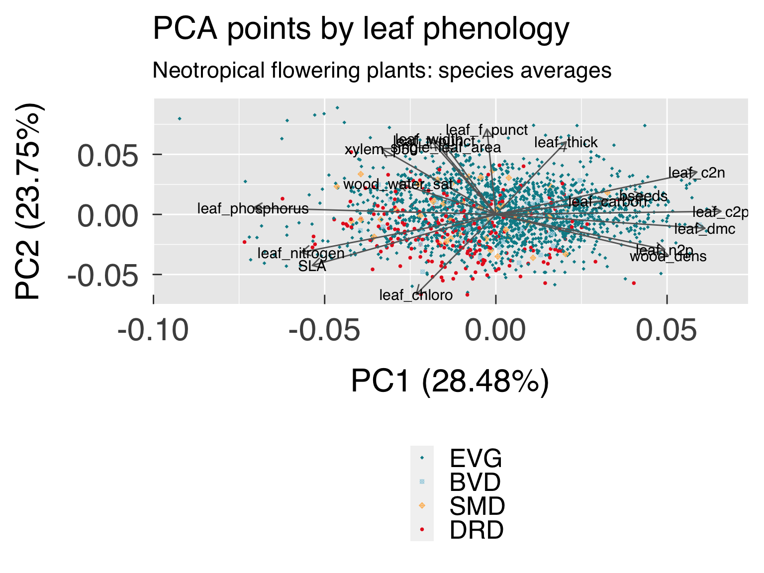
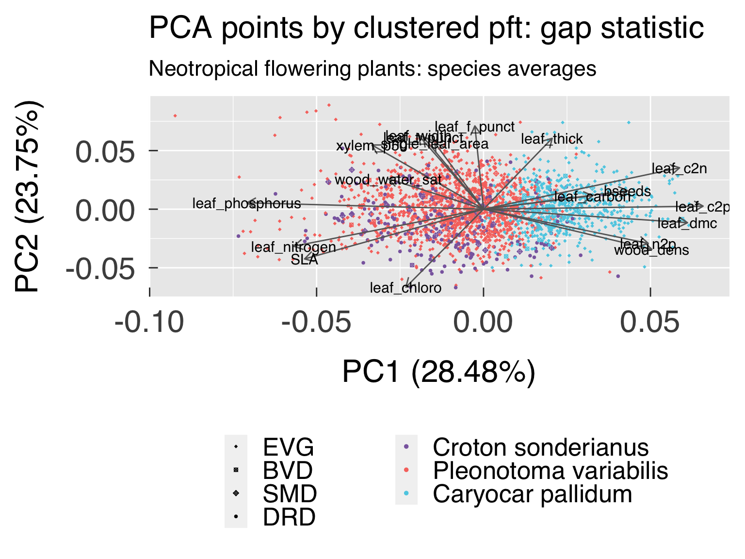
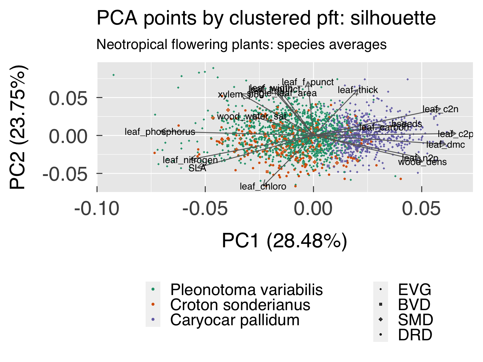
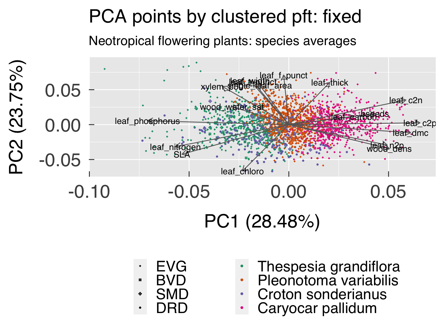
Plot the medoid of all variables used in the cluster analysis
Here we plot the medoid of each cluster for all traits included as a
radial plot, which is obtained by finding the equivalent value of the
CDF for each trait.
if (plot_radar_cluster){
   cat0(" + Plot radar plot for medoids.")
   # Retrieve medoid values and select traits that are numeric and have a global distribution.
   HasDistrib = names(MedoidTRY)[names(MedoidTRY) %in% GlobDistr$x   ]
   IsTrait    = names(MedoidTRY)[names(MedoidTRY) %in% try_trait$Name]
   NormalLoop = sort(intersect(HasDistrib,IsTrait))
   KeepMedoid = unique(c("Cluster",NormalLoop))


   RadarTRY = MedoidTRY %>%
      select(all_of(KeepMedoid))

   # Loop through the numeric variables and find the CDF.
   for (v in seq_along(NormalLoop)){
      # Retrieve information for this variable
      vName   = NormalLoop[v]
      vIndex  = match(vName,GlobDistr$x)
      vDistr  = GlobDistr$Distrib[vIndex]
      vFirst  = GlobDistr$First  [vIndex]
      vSecond = GlobDistr$Second [vIndex]
      vThird  = GlobDistr$Third  [vIndex]

      # Fit the cumulative density function according to the distribution.
      vFun = switch( vDistr
                   , "uniform"       = punif
                   , "normal"        = pnorm
                   , "logistic"      = plogis
                   , "skew-normal"   = sn::psn
                   , "log-normal"    = plnorm
                   , "neglog-normal" = pnlnorm
                   , "weibull"       = pweibull
                   , "gamma"         = pgamma
                   , NA_character_
                   )#end switch

      # Decide whether the distribution needs two or three parameters
      if (vDistr %in% "skew-normal"){
         RadarTRY[[vName]] = vFun(RadarTRY[[vName]],vFirst,vSecond,vThird)
      }else if (! is.na(zDistr)){
         RadarTRY[[vName]] = vFun(RadarTRY[[vName]],vFirst,vSecond)
      }#end if (zDistr %in% "skew-normal")

      # Delete NaN values
      RadarTRY[[vName]] = ifelse( test = is.finite(RadarTRY[[vName]])
                                , yes  = RadarTRY[[vName]]
                                , no   = NA_real_
                                )#end ifelse
   }#end for (v in seq_along(NormalLoop))

   # Create a table abbreviations
   NormalAbbr        = letters[seq_along(NormalLoop)]
   names(NormalAbbr) = NormalLoop

   # List of classes for ordering the clusters. We add "All" as a dummy cluster
   CategUse   = CategExtra %>% filter((TraitID %in% 0) | (Class %in% "ALL"))
   orderCateg = c(nrow(CategUse),sequence(nrow(CategUse)-1L))
   CategUse   = CategUse[orderCateg,]

   # Append a column with all, which will be used as a legend
   AppendTRY = RadarTRY[1L,,drop=FALSE] %>%
      mutate( across(where(is.numeric), ~ NA_real_ * .x)
            , Cluster = CategUse$Class[1L])

   RadarTRY = rbind(AppendTRY,RadarTRY)


   # Reshape RadarTRY so the variables become a categorical variable
   RadarPlot = RadarTRY %>%
      pivot_longer(all_of(NormalLoop),names_to="Variable",values_to="CumDistr") %>%
      mutate( Cluster  = factor(x=Cluster,levels=CategUse$Class)
            , Variable = factor(x=Variable,levels=NormalLoop,labels=NormalAbbr) )


   gg_radar = ggplot( data = RadarPlot, mapping = aes(x=Variable,y=CumDistr,group=Cluster) )
   gg_radar = gg_radar + facet_wrap( ~Cluster, nrow=2L)
   gg_radar = gg_radar + geom_polygon(colour="#1F78B4",fill="#A6CEE3",alpha=0.7,linewidth=I(1.2))
   gg_radar = gg_radar + geom_hline(yintercept=c(0.25,0.5,0.75),colour="black",linetype="dotted",linewidth=I(0.3))
   gg_radar = gg_radar + geom_hline(yintercept=c(1.0),colour="black",linetype="solid",linewidth=I(0.3))
   gg_radar = gg_radar + scale_y_continuous(limits=c(0.,1.0),breaks=c(0.,0.25,0.5,0.75,1.0))
   gg_radar = gg_radar + coord_curvedpolar()

   gg_radar = gg_radar + labs( x        = element_blank()
                             , y        = element_blank()
                             , title    = "Relative traits for the cluster medoids"
                             , subtitle = LabelSubtitle
                             )#end labs
   gg_radar = gg_radar + theme_grey( base_size = gg_ptsz, base_family = "Helvetica",base_line_size = 0.5,base_rect_size =0.5)
   gg_radar = gg_radar + theme( axis.text.x       = element_text( size = gg_ptsz, margin = unit(rep(0.35,times=4),"cm"))
                              , axis.text.y       = element_blank()
                              , axis.ticks.y      = element_blank()
                              , plot.title        = element_text( size = gg_ptsz)
                              , plot.subtitle     = element_text( size = 0.7*gg_ptsz)
                              , axis.ticks.length = unit(-0.25,"cm")
                              , legend.position   = "bottom"
                              , legend.direction  = "horizontal"
                              )#end theme
   # Save plot in every format requested.
   for (d in sequence(ndevice)){
      f_output = paste0("RadarPlot_Faceted_",base_suffix,".",gg_device[d])
      dummy = ggsave( filename = f_output
                    , plot     = gg_radar
                    , device   = gg_device[d]
                    , path     = trpca_path
                    , width    = gg_width
                    , height   = gg_height
                    , units    = gg_units
                    , dpi      = gg_depth
                    )#end ggsave
   }#end for (o in sequence(nout))

   # If sought, plot images on screen
   if (gg_screen) gg_radar
}#end if (plot_radar_cluster)
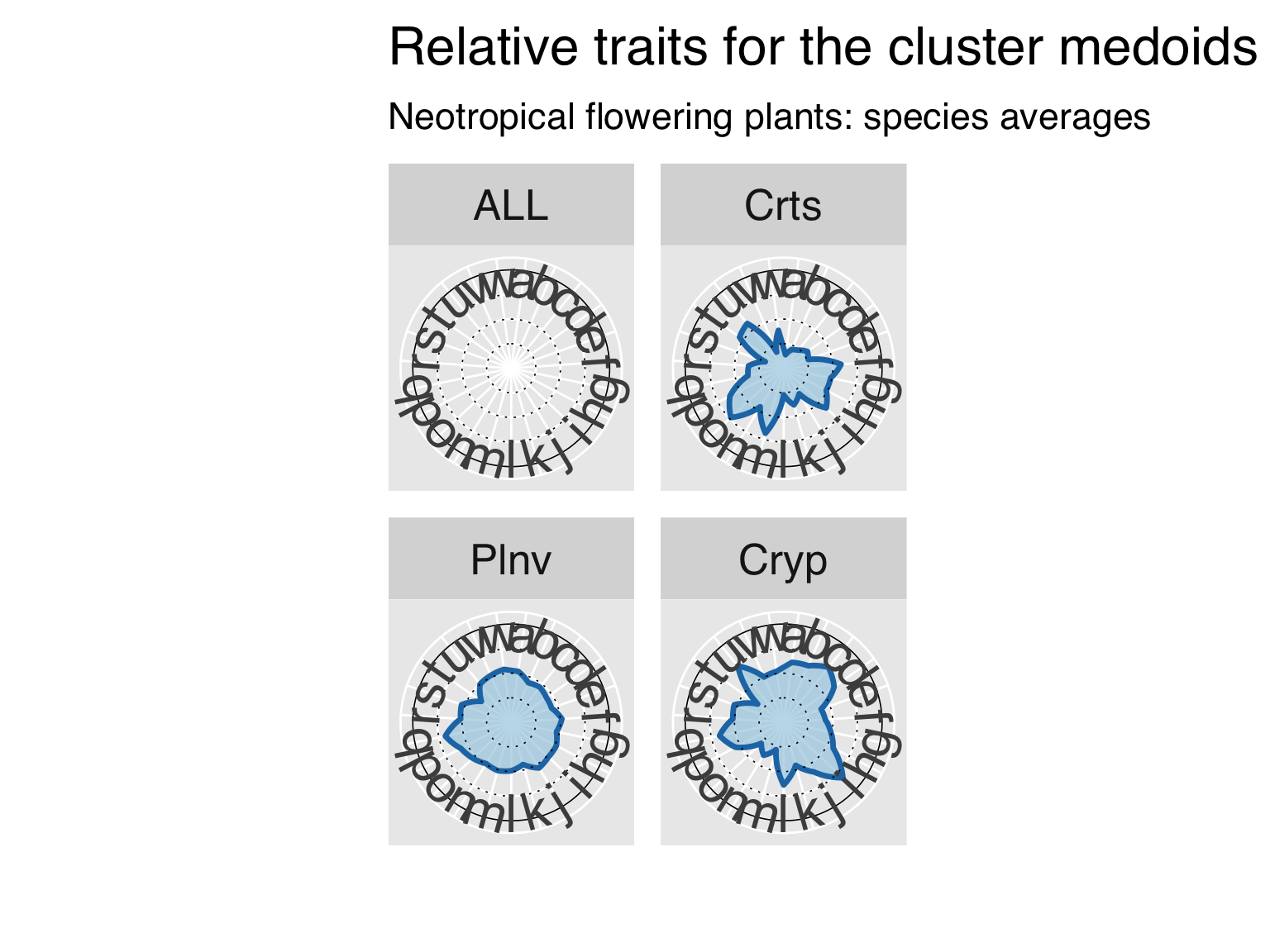
Plot trait trade-off relationships
In this part, we plot the standardised major axis fit for all trait
pairs, accounting for trait variation flagged as “colour”, in addition
to the trade-offs distinguished by data-based clusters.
# Select reference data set for trade-off analysis
DataTRY = switch( EXPR       = fit_taxon
                , Individual = TidyTRY
                , Species    = SpeciesTRY
                , Genus      = GenusTRY
                , stop("Invalid settings for variable \"fit_taxon\".")
                )#end switch

# Load settings for the x axis.
x      = xsma_idx
xTrait = try_trait$TraitID[x]
xName  = try_trait$Name   [x]
xDesc  = try_trait$Desc   [x]
xUnit  = try_trait$Unit   [x]
xTrans = try_trait$Trans  [x]
xTPlot = switch( EXPR = xTrans, log = "log10", neglog="neglog10",xTrans)

# Select valid data for the y axis
xSel = switch( EXPR     = xTrans
             , identity = is.finite(DataTRY[[xName]])
             , log      = DataTRY[[xName]] %gt% 0.
             , neglog   = DataTRY[[xName]] %lt% 0.
             , sqrt     = DataTRY[[xName]] %ge% 0.
             , cbrt     = is.finite(DataTRY[[xName]])
             , stop(paste0(" Invalid transformation for trait ",xName," (TraitID = ",xTrait,")."))
             )#end switch


# Find out how many SMA fits we will seek
yPlotSMA = which(try_trait$SMA & (! (try_trait$Name %in% xName)))
CntSMA   = length(yPlotSMA)


# Initialise the list of plots
gg_SMA = list()

# Find the number of traits for plotting the model
CategSel    = is.finite(CategSMA$TraitID) & plot_sma_trait
CategTrait  = sort(unique(CategSMA$TraitID[CategSel]))
for (ct in seq_along(CategTrait)){
   # Load settings for the classes.
   zTrait = CategTrait[ct]
   if (zTrait %in% 0L){
      zName  = "Cluster"
      zDesc  = "Data-based cluster class"
   }else{
      z      = match(zTrait,try_trait$TraitID)
      zName  = try_trait$Name   [z]
      zDesc  = try_trait$Desc   [z]
   }#end if (zTrait %in% 0L)
   zTitle = paste0("SMA model by ",tolower(zDesc))

   # Set path for this group of plots.
   categ_trsma_path = file.path(trsma_path,zName)


   # Select categories for this trait type.
   CategNow = CategExtra %>%
      filter( (TraitID %in% zTrait) | is.na(TraitID)) %>%
      filter((! duplicated(Class)))

   CntCategNow = nrow(CategNow)


   # Loop through the SMA variables
   for (y in sequence(CntSMA)){
      # Load settings for the y axis.
      yIndex = yPlotSMA[y]
      yTrait = try_trait$TraitID[yIndex]
      yName  = try_trait$Name   [yIndex]
      yLower = paste0(yName,"_Lower")
      yUpper = paste0(yName,"_Upper")
      yDesc  = try_trait$Desc   [yIndex]
      yUnit  = try_trait$Unit   [yIndex]
      yTrans = try_trait$Trans  [yIndex]
      yTPlot = switch( EXPR = yTrans, log = "log10", neglog="neglog10",yTrans)

      # Select valid data for the y axis
      ySel = switch( EXPR     = yTrans
                   , identity = is.finite(DataTRY[[yName]])
                   , log      = DataTRY[[yName]] %gt% 0.
                   , neglog   = DataTRY[[yName]] %lt% 0.
                   , sqrt     = DataTRY[[yName]] %ge% 0.
                   , cbrt     = is.finite(DataTRY[[yName]])
                   , stop(paste0(" Invalid transformation for trait ",yName," (TraitID = ",yTrait,")."))
                   )#end switch

      # Subset data
      DataPlot = DataTRY %>%
         filter(xSel & ySel) %>%
         select_at(vars(c(xName,yName,zName))) %>%
         mutate_at( vars(c(zName)), ~ifelse(.x %in% CategNow$Class,.x,"UKN")) %>%
         mutate_at( vars(c(zName)), ~factor(.x,levels=CategNow$Class))
      PlotSMA  = nrow(DataPlot) %ge% n_fit_min

      # Append dummy data with category ALL so legends can be merged.
      DataDummy = DataPlot[rep(1L,times=CntCategNow),,drop=FALSE] %>%
         mutate(across(c(xName,yName), ~ c(NA_real_))) %>%
         mutate(across(c(zName), ~ factor(CategNow$Class,levels=CategNow$Class) ) )
      DataPlot    = rbind(DataPlot,DataDummy)
      CntDataPlot = nrow(DataPlot)

      # Plot only the variables with meaningful data
      if (PlotSMA){
         cat0(" + Plot the trait trade-offs (and SMA fits) for ",yDesc,", by ",zDesc,".")


         # Set path for this group of plots.
         dummy = dir.create(categ_trsma_path,recursive=TRUE,showWarnings=FALSE)


         # Find limits for plots.
         xLimit = range(DataPlot[[xName]],finite=TRUE)
         yLimit = range(DataPlot[[yName]],finite=TRUE)


         # Subset predicted data, so the range is consistent with the subset data:
         pSel     = ( ( (PredSMA[[xName]] %wr% xLimit) | is.na(PredSMA[[xName]]) )
                    & ( (PredSMA[[yName]] %wr% yLimit) | is.na(PredSMA[[yName]]) )
                    & (PredSMA$TraitClass %in% c("All","Unknown",zName)) )
         PredPlot = PredSMA %>%
            filter(pSel)    %>%
            mutate(Class = factor(Class,levels = CategNow$Class)) %>%
            rename_at( vars(c("Class")), ~ c(zName)) %>%
            select_at(vars(c(xName,yName,zName)))
         PlotFit  = any(is.finite(PredPlot[[yName]]))


         # Subset SMA summary
         InfoPlot = InfoSMA %>%
            filter( (x %in% xName) & (y %in% yName) & ( TraitClass %in% c("All",zName) ) ) %>%
            select( ! TraitClass) %>%
            rename_at( vars(c("Class")), ~ c(zName)) %>%
            add_row("{zName}" := "UKN") %>%
            mutate( across(c(zName), ~ factor(.x,levels = CategNow$Class))) %>%
            mutate( across(c("x","y","xTrans","yTrans"), ~ ifelse(test=is.na(.x),yes=commonest(.x,na.rm=TRUE),no=.x))
                  , N      = ifelse(test=is.na(N),yes=0L,no=N)
                  , Line   = cut(pValue,breaks=c(0,0.001,0.01,0.05,0.10,1),labels=FALSE)
                  , Line   = ifelse( test = is.na(Line)
                                   , yes  = "blank"
                                   , no   = c("solid","dotdash","dashed","dotted","blank")[Line]
                                   )#end ifelse
                  )#end mutate

         # Set categories for colours, lines and symbols
         colClasses        = CategNow$Colour
         names(colClasses) = CategNow$Class
         pchClasses        = CategNow$Symbol
         names(pchClasses) = CategNow$Class
         ltyClasses        = InfoPlot$Line
         names(ltyClasses) = InfoPlot[[zName]]
         ltyClasses        = ltyClasses[match(names(pchClasses),names(ltyClasses))]


         # Build the plot
         gg_now = ggplot()
         gg_now = gg_now + geom_point(data=DataPlot,aes_string(x=xName,y=yName,colour=zName,shape=zName),size=1.9)
         gg_now = gg_now + scale_colour_manual  (values=colClasses)
         gg_now = gg_now + scale_shape_manual   (values=pchClasses)
         if (PlotFit){
            #gg_now = gg_now + geom_ribbon(data=PredPlot,aes_string(x=xName,ymin=yLower,ymax=yUpper,fill=zName),alpha=0.35,colour="transparent")
            gg_now = gg_now + scale_fill_manual(values=colClasses)
            gg_now = gg_now + geom_line(data=PredPlot,aes_string(x=xName,y=yName,colour=zName,linetype=zName),size=1.25,inherit.aes = FALSE)
            gg_now = gg_now + scale_linetype_manual(values=ltyClasses)
            gg_now = gg_now + labs( x        = desc.unit(desc=xDesc,unit=untab[[xUnit]])
                                  , y        = desc.unit(desc=yDesc,unit=untab[[yUnit]])
                                  , colour   = element_blank()
                                  , fill     = element_blank()
                                  , shape    = element_blank()
                                  , linetype = element_blank()
                                  , title    = zTitle
                                  , subtitle = LabelSubtitle
                                  )#end labs
         }else{
            gg_now = gg_now + labs( x        = desc.unit(desc=xDesc,unit=untab[[xUnit]])
                                  , y        = desc.unit(desc=yDesc,unit=untab[[yUnit]])
                                  , colour   = element_blank()
                                  , shape    = element_blank()
                                  , title    = zTitle
                                  , subtitle = LabelSubtitle
                                  )#end labs
         }#end if (PlotFit)
         gg_now = gg_now + theme_grey( base_size = gg_ptsz, base_family = "Helvetica",base_line_size = 0.5,base_rect_size =0.5)
         gg_now = gg_now + theme( axis.text.x       = element_text( size = gg_ptsz, margin = unit(rep(0.35,times=4),"cm"))
                                , axis.text.y       = element_text( size = gg_ptsz, margin = unit(rep(0.35,times=4),"cm"))
                                , plot.title        = element_text( size = gg_ptsz)
                                , plot.subtitle     = element_text( size = 0.7*gg_ptsz)
                                , axis.ticks.length = unit(-0.25,"cm")
                                , legend.position   = "bottom"
                                , legend.direction  = "horizontal"
                                )#end theme
         gg_now = gg_now + scale_x_continuous(trans=xTPlot,limits=xLimit)
         gg_now = gg_now + scale_y_continuous(trans=yTPlot,limits=yLimit)
         #      gg_now = gg_now + coord_trans(x=xTPlot,y=yTPlot,xlim=xLimit,ylim=yLimit)

         # Save plot in every format requested.
         for (d in sequence(ndevice)){
            f_output = paste0("SMAPlot_",yName,"_by-",zName,"_",trait_suffix,".",gg_device[d])
            dummy    = ggsave( filename = f_output
                             , plot     = gg_now
                             , device   = gg_device[d]
                             , path     = categ_trsma_path
                             , width    = gg_square
                             , height   = gg_square
                             , units    = gg_units
                             , dpi      = gg_depth
                             )#end ggsave
         }#end for (o in sequence(nout))

         # Write plot settings to the list.
         yzName           = paste0(yName,"_",zName)
         gg_SMA[[yzName]] = gg_now
      }else{
         cat0(" + Skip plot for ",yDesc," by ",zDesc,": too few valid points.")

      }#end if (PlotSMA)
   }#end for (y in yloop)
}#end for (z in seq_along(CategTrait))

# If sought, plot images on screen
cnt_gg_SMA = length(gg_SMA)
if (gg_screen && (cnt_gg_SMA %gt% 0L)){
   gg_show = sort(sample.int(n=cnt_gg_SMA,size=min(cnt_gg_SMA,3L),replace=FALSE))
   gg_SMA[gg_show]
}#end if (gg_screen && (length(gg_SMA) %gt% 0L))
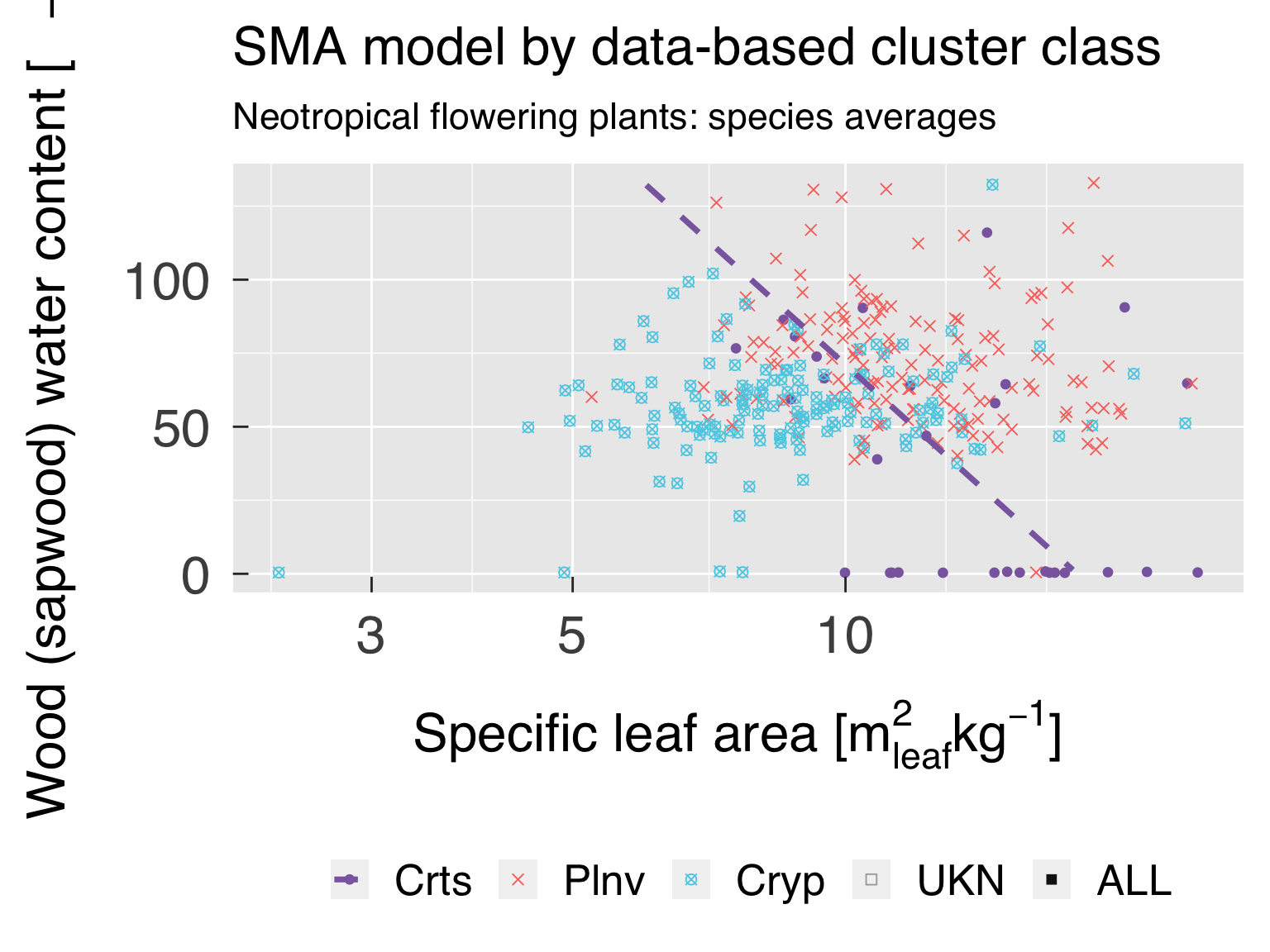
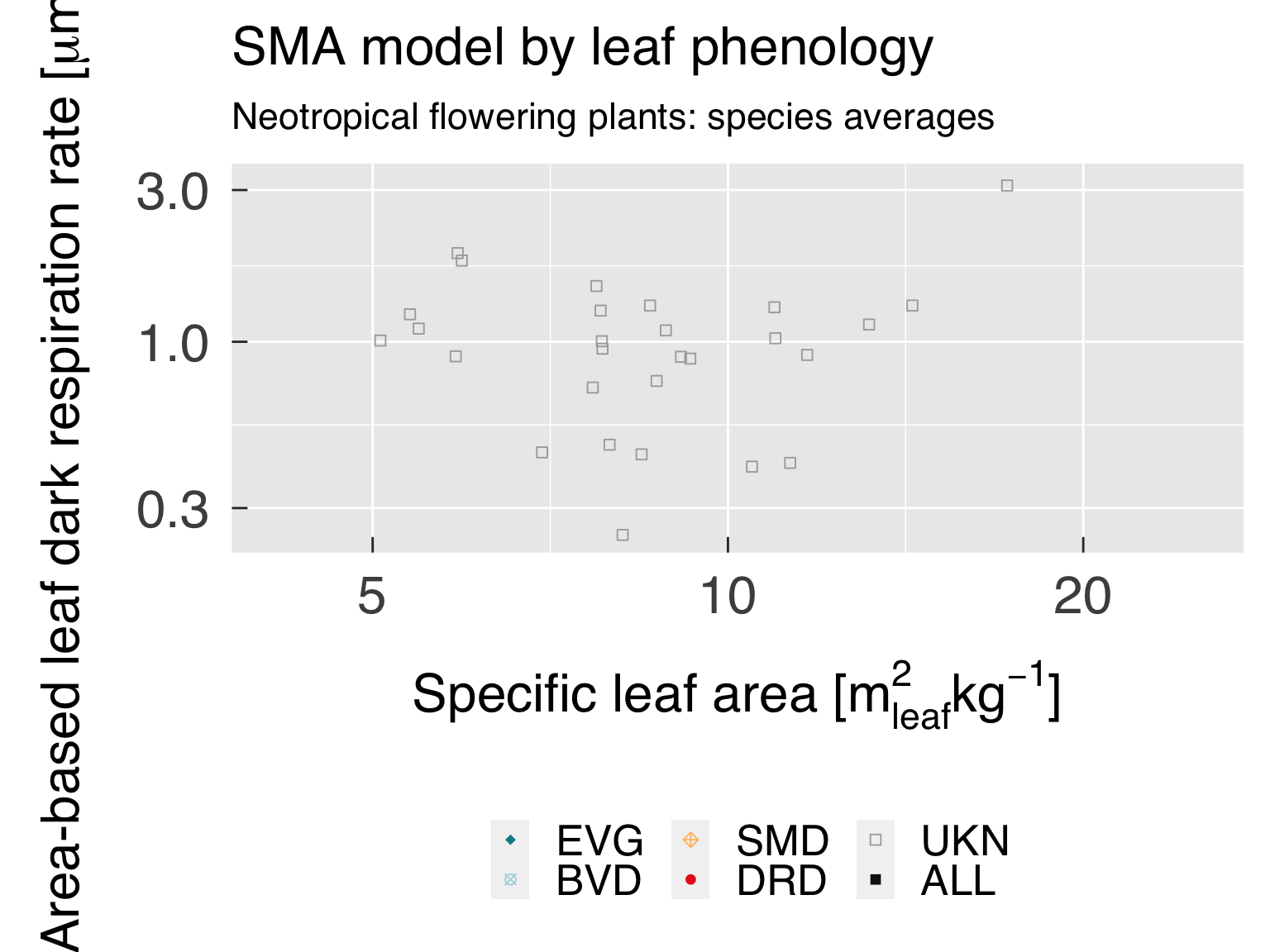
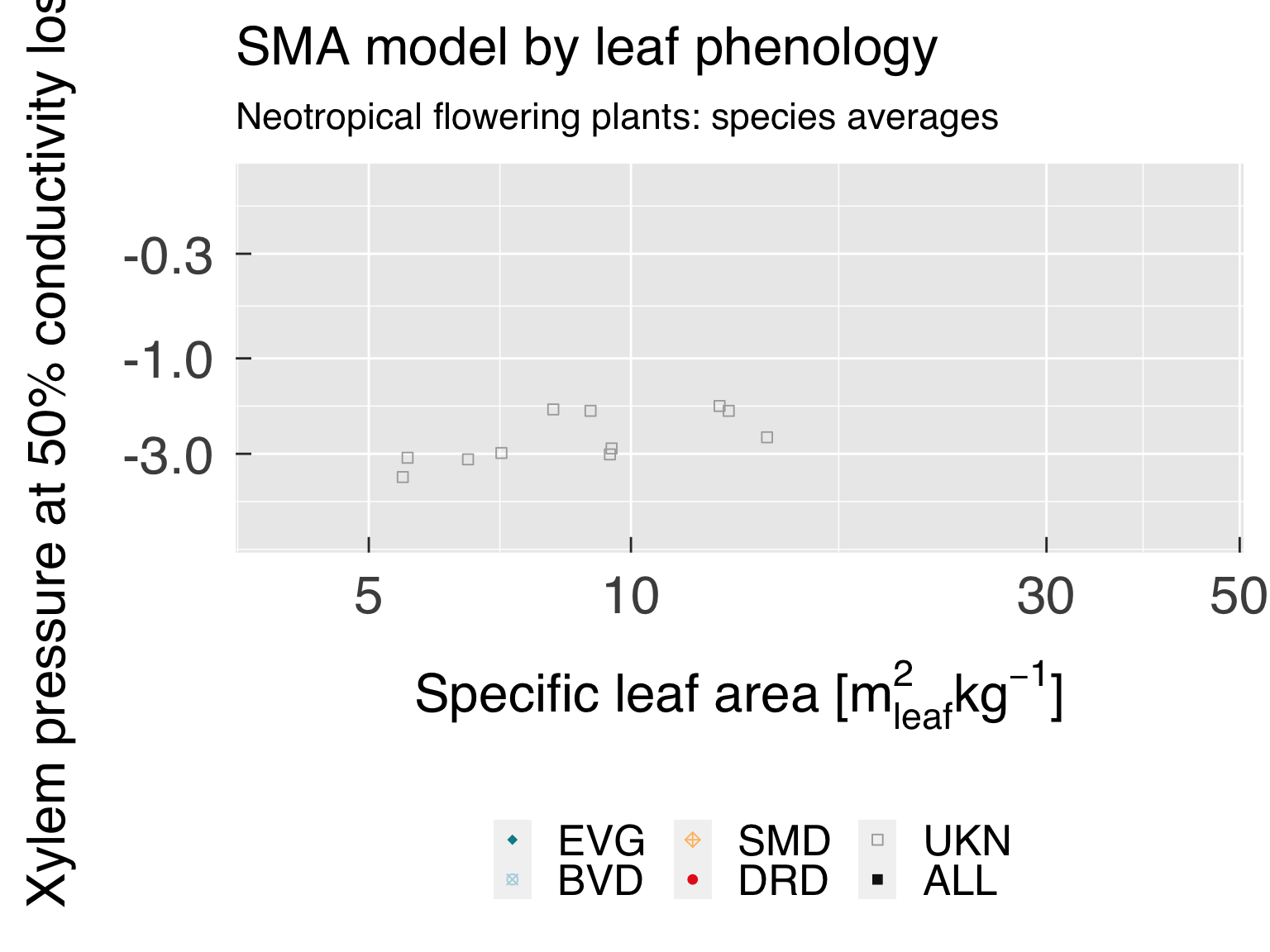
And in this block, we do the same for the photosynthetic traits.
# Select reference data set for trade-off analysis
DataTRY = switch( EXPR       = fit_taxon
                , Individual = TidyTRY
                , Species    = SpeciesTRY
                , Genus      = GenusTRY
                , stop("Invalid settings for variable \"fit_taxon\".")
                )#end switch

# Load settings for the x axis.
x      = xphoto_idx
xTrait = try_trait$TraitID[x]
xName  = try_trait$Name   [x]
xDesc  = try_trait$Desc   [x]
xUnit  = try_trait$Unit   [x]
xTrans = try_trait$Trans  [x]
xTPlot = switch( EXPR = xTrans, log = "log10", neglog="neglog10",xTrans)

# Select valid data for the y axis
xSel = switch( EXPR     = xTrans
             , identity = is.finite(DataTRY[[xName]])
             , log      = DataTRY[[xName]] %gt% 0.
             , neglog   = DataTRY[[xName]] %lt% 0.
             , sqrt     = DataTRY[[xName]] %ge% 0.
             , cbrt     = is.finite(DataTRY[[xName]])
             , stop(paste0(" Invalid transformation for trait ",xName," (TraitID = ",xTrait,")."))
             )#end switch


# Find out how many SMA (Photosynthesis) fits we will seek
yPlotPhoto = which(try_trait$SMA & try_trait$Photo & (! (try_trait$Name %in% xName)))
CntPhoto   = length(yPlotPhoto)

# Initialise the list of plots
gg_Photo = list()

# Find the number of traits for plotting the model
CategSel    = is.finite(CategPhoto$TraitID) & plot_sma_photo
CategTrait  = sort(unique(CategPhoto$TraitID[CategSel]))
for (ct in seq_along(CategTrait)){
   # Load settings for the classes.
   zTrait = CategTrait[ct]
   if (zTrait %in% 0L){
      zName  = "Cluster"
      zDesc  = "Data-based cluster class"
   }else{
      z      = match(zTrait,try_trait$TraitID)
      zName  = try_trait$Name   [z]
      zDesc  = try_trait$Desc   [z]
   }#end if (zTrait %in% 0L)
   zTitle = paste0("SMA model by ",tolower(zDesc))

   # Set path for this group of plots.
   categ_photo_path = file.path(photo_path,zName)


   # Select categories for this trait type.
   CategNow = CategExtra %>%
      filter( (TraitID %in% zTrait) | is.na(TraitID)) %>%
      filter((! duplicated(Class)))

   CntCategNow = nrow(CategNow)


   # Loop through the SMA (Photosynthesis) variables
   for (y in sequence(CntPhoto)){
      # Load settings for the y axis.
      yIndex = yPlotPhoto[y]
      yTrait = try_trait$TraitID[yIndex]
      yName  = try_trait$Name   [yIndex]
      yLower = paste0(yName,"_Lower")
      yUpper = paste0(yName,"_Upper")
      yDesc  = try_trait$Desc   [yIndex]
      yUnit  = try_trait$Unit   [yIndex]
      yTrans = try_trait$Trans  [yIndex]
      yTPlot = switch( EXPR = yTrans, log = "log10", neglog="neglog10",yTrans)

      # Select valid data for the y axis
      ySel = switch( EXPR     = yTrans
                   , identity = is.finite(DataTRY[[yName]])
                   , log      = DataTRY[[yName]] %gt% 0.
                   , neglog   = DataTRY[[yName]] %lt% 0.
                   , sqrt     = DataTRY[[yName]] %ge% 0.
                   , cbrt     = is.finite(DataTRY[[yName]])
                   , stop(paste0(" Invalid transformation for trait ",yName," (TraitID = ",yTrait,")."))
                   )#end switch

      # Subset data
      DataPlot = DataTRY %>%
         filter(xSel & ySel) %>%
         select_at(vars(c(xName,yName,zName))) %>%
         mutate_at( vars(c(zName)), ~ifelse(.x %in% CategNow$Class,.x,"UKN")) %>%
         mutate_at( vars(c(zName)), ~factor(.x,levels=CategNow$Class))
      PlotPhoto  = nrow(DataPlot) %ge% n_fit_min

      # Append dummy data with category ALL so legends can be merged.
      DataDummy = DataPlot[rep(1L,times=CntCategNow),,drop=FALSE] %>%
         mutate(across(c(xName,yName), ~ c(NA_real_))) %>%
         mutate(across(c(zName), ~ factor(CategNow$Class,levels=CategNow$Class) ) )
      DataPlot    = rbind(DataPlot,DataDummy)
      CntDataPlot = nrow(DataPlot)

      # Plot only the variables with meaningful data
      if (PlotPhoto){
         cat0(" + Plot the trait trade-offs (and SMA fits) for ",yDesc,", by ",zDesc,".")


         # Set path for this group of plots.
         dummy = dir.create(categ_photo_path,recursive=TRUE,showWarnings=FALSE)


         # Find limits for plots.
         xLimit = range(DataPlot[[xName]],finite=TRUE)
         yLimit = range(DataPlot[[yName]],finite=TRUE)


         # Subset predicted data, so the range is consistent with the subset data:
         pSel     = ( ( (PredPhoto[[xName]] %wr% xLimit) | is.na(PredPhoto[[xName]]) )
                    & ( (PredPhoto[[yName]] %wr% yLimit) | is.na(PredPhoto[[yName]]) )
                    & (PredPhoto$TraitClass %in% c("All","Unknown",zName)) )
         PredPlot = PredPhoto %>%
            filter(pSel)    %>%
            mutate(Class = factor(Class,levels = CategNow$Class)) %>%
            rename_at( vars(c("Class")), ~ c(zName)) %>%
            select_at(vars(c(xName,yName,zName)))
         PlotFit  = any(is.finite(PredPlot[[yName]]))


         # Subset SMA (Photosynthesis) summary
         InfoPlot = InfoPhoto %>%
            filter( (x %in% xName) & (y %in% yName) & ( TraitClass %in% c("All",zName) ) ) %>%
            select( ! TraitClass) %>%
            rename_at( vars(c("Class")), ~ c(zName)) %>%
            add_row("{zName}" := "UKN") %>%
            mutate( across(c(zName), ~ factor(.x,levels = CategNow$Class))) %>%
            mutate( across(c("x","y","xTrans","yTrans"), ~ ifelse(test=is.na(.x),yes=commonest(.x,na.rm=TRUE),no=.x))
                  , N      = ifelse(test=is.na(N),yes=0L,no=N)
                  , Line   = cut(pValue,breaks=c(0,0.001,0.01,0.05,0.10,1),labels=FALSE)
                  , Line   = ifelse( test = is.na(Line)
                                   , yes  = "blank"
                                   , no   = c("solid","dotdash","dashed","dotted","blank")[Line]
                                   )#end ifelse
                  )#end mutate

         # Set categories for colours, lines and symbols
         colClasses        = CategNow$Colour
         names(colClasses) = CategNow$Class
         pchClasses        = CategNow$Symbol
         names(pchClasses) = CategNow$Class
         ltyClasses        = InfoPlot$Line
         names(ltyClasses) = InfoPlot[[zName]]
         ltyClasses        = ltyClasses[match(names(pchClasses),names(ltyClasses))]


         # Build the plot
         gg_now = ggplot()
         gg_now = gg_now + geom_point(data=DataPlot,aes_string(x=xName,y=yName,colour=zName,shape=zName),size=1.6)
         gg_now = gg_now + scale_colour_manual  (values=colClasses)
         gg_now = gg_now + scale_shape_manual   (values=pchClasses)
         if (PlotFit){
            #gg_now = gg_now + geom_ribbon(data=PredPlot,aes_string(x=xName,ymin=yLower,ymax=yUpper,fill=zName),alpha=0.35,colour="transparent")
            gg_now = gg_now + scale_fill_manual(values=colClasses)
            gg_now = gg_now + geom_line(data=PredPlot,aes_string(x=xName,y=yName,colour=zName,linetype=zName),size=1.25,inherit.aes = FALSE)
            gg_now = gg_now + scale_linetype_manual(values=ltyClasses)
            gg_now = gg_now + labs( x        = desc.unit(desc=xDesc,unit=untab[[xUnit]])
                                  , y        = desc.unit(desc=yDesc,unit=untab[[yUnit]])
                                  , colour   = element_blank()
                                  , fill     = element_blank()
                                  , shape    = element_blank()
                                  , linetype = element_blank()
                                  , title    = zTitle
                                  , subtitle = LabelSubtitle
                                  )#end labs
         }else{
            gg_now = gg_now + labs( x        = desc.unit(desc=xDesc,unit=untab[[xUnit]])
                                  , y        = desc.unit(desc=yDesc,unit=untab[[yUnit]])
                                  , colour   = element_blank()
                                  , shape    = element_blank()
                                  , title    = zTitle
                                  , subtitle = LabelSubtitle
                                  )#end labs
         }#end if (PlotFit)
         gg_now = gg_now + theme_grey( base_size = gg_ptsz, base_family = "Helvetica",base_line_size = 0.5,base_rect_size =0.5)
         gg_now = gg_now + theme( axis.text.x       = element_text( size = gg_ptsz, margin = unit(rep(0.35,times=4),"cm"))
                                , axis.text.y       = element_text( size = gg_ptsz, margin = unit(rep(0.35,times=4),"cm"))
                                , plot.title        = element_text( size = gg_ptsz)
                                , plot.subtitle     = element_text( size = 0.7*gg_ptsz)
                                , axis.ticks.length = unit(-0.25,"cm")
                                , legend.position   = "bottom"
                                , legend.direction  = "horizontal"
                                )#end theme
         gg_now = gg_now + scale_x_continuous(trans=xTPlot,limits=xLimit)
         gg_now = gg_now + scale_y_continuous(trans=yTPlot,limits=yLimit)
         #      gg_now = gg_now + coord_trans(x=xTPlot,y=yTPlot,xlim=xLimit,ylim=yLimit)

         # Save plot in every format requested.
         for (d in sequence(ndevice)){
            f_output = paste0("SMAPlot_",yName,"_by-",zName,"_",photo_suffix,".",gg_device[d])
            dummy    = ggsave( filename = f_output
                             , plot     = gg_now
                             , device   = gg_device[d]
                             , path     = categ_photo_path
                             , width    = gg_width
                             , height   = gg_height
                             , units    = gg_units
                             , dpi      = gg_depth
                             )#end ggsave
         }#end for (o in sequence(nout))

         # Write plot settings to the list.
         yzName             = paste0(yName,"_",zName)
         gg_Photo[[yzName]] = gg_now
      }else{
         cat0(" + Skip plot for ",yDesc," by ",zDesc,": too few valid points.")

      }#end if (PlotPhoto)
   }#end for (y in yloop)
}#end for (z in seq_along(CategTrait))

# If sought, plot images on screen
cnt_gg_Photo = length(gg_Photo)
if (gg_screen && (cnt_gg_Photo %gt% 0L)){
   gg_show = sort(sample.int(n=cnt_gg_Photo,size=min(cnt_gg_Photo,3L),replace=FALSE))
   gg_Photo[gg_show]
}#end if (gg_screen && (length(gg_Photo) %gt% 0L))
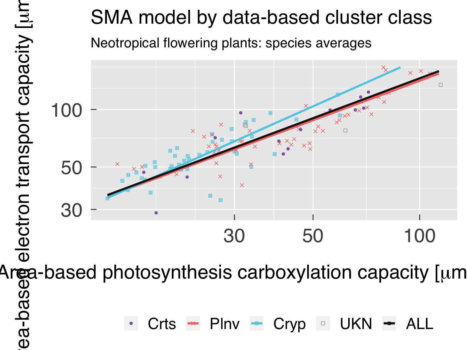
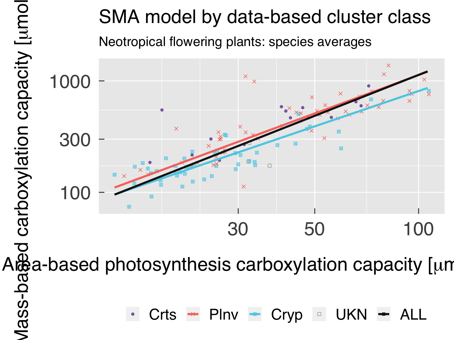
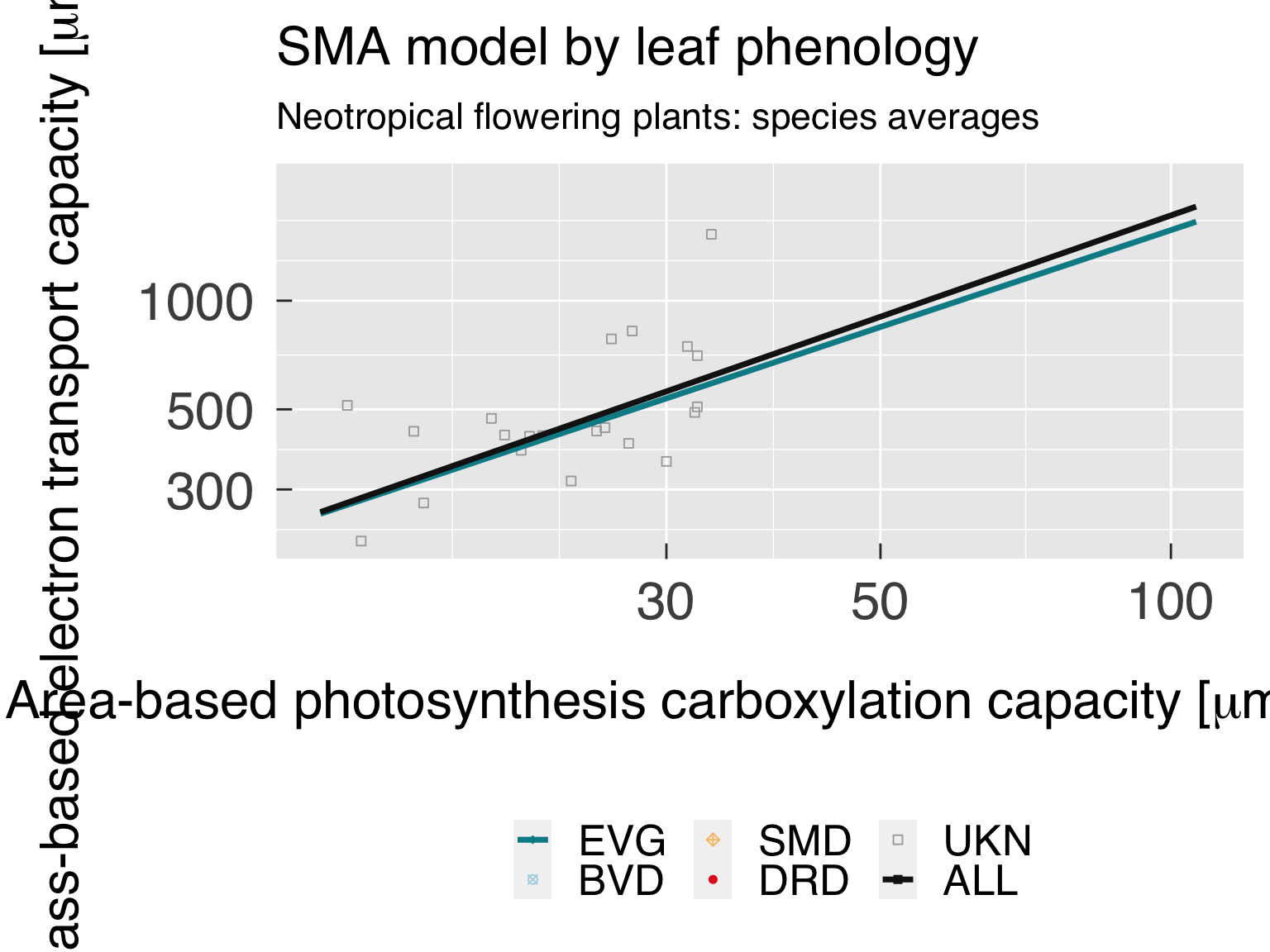
Plot global trait distribution
Here we plot the global trait distribution as a separate set, which
can be useful for some analyses.
# Select reference data set for trade-off analysis
DataTRY    = switch( EXPR       = fit_taxon
                   , Individual = TidyTRY
                   , Species    = SpeciesTRY
                   , Genus      = GenusTRY
                   , stop("Invalid settings for variable \"fit_taxon\".")
                   )#end switch

# Set path for this group of plots.
global_trdist_path = file.path(trdist_path,"Global")

# Select distribution statistics for this trait type
InfoNow = InfoDistr %>%
   filter(TraitClass %in% c("All")) %>%
   select(! c(Class,TraitClass)) %>%
   mutate(Label = NA_character_)

# Find out how many distribution plots we will make
xPlotDistr = which(try_trait$SMA & (try_trait$Name %in% InfoDistr$x) & plot_global_distrib)
CntDistr   = length(xPlotDistr)

# Initialise list with plots
gg_Distr = list()

# Loop through the SMA variables
for (x in sequence(CntDistr)){
   # Load settings for the y axis.
   xIndex    = xPlotDistr[x]
   xTrait    = try_trait$TraitID[xIndex]
   xName     = try_trait$Name   [xIndex]
   xLower    = paste0(yName,"_Lower")
   xUpper    = paste0(yName,"_Upper")
   xDesc     = try_trait$Desc   [xIndex]
   xUnit     = try_trait$Unit   [xIndex]
   xTrans    = try_trait$Trans  [xIndex]
   xTPlot    = switch( EXPR = xTrans, log = "log10", neglog="neglog10",xTrans)
   xInfo     = which(InfoNow$x %in% xName)
   xDistr    = InfoNow$Distrib[xInfo]
   xFirst    = InfoNow$First  [xInfo]
   xSecond   = InfoNow$Second [xInfo]
   xThird    = InfoNow$Third  [xInfo]
   xColLine  = RColorBrewer::brewer.pal(n=2L,name="Paired")[2L]
   xColPoint = RColorBrewer::brewer.pal(n=2L,name="Paired")[1L]


   # Select valid data for the x axis
   xSel = switch( EXPR     = xTrans
                , identity = is.finite(DataTRY[[xName]])
                , log      = DataTRY[[xName]] %gt% 0.
                , neglog   = DataTRY[[xName]] %lt% 0.
                , sqrt     = DataTRY[[xName]] %ge% 0.
                , cbrt     = is.finite(DataTRY[[xName]])
                , stop(paste0(" Invalid transformation for trait ",xName," (TraitID = ",xTrait,")."))
                )#end switch

   # Fit density according to the distribution.
   xFun = switch( xDistr
                , "uniform"       = dunif
                , "normal"        = dnorm
                , "logistic"      = dlogis
                , "skew-normal"   = sn::dsn
                , "log-normal"    = dlnorm
                , "neglog-normal" = dnlnorm
                , "weibull"       = dweibull
                , "gamma"         = dgamma
                , NA_character_
                )#end switch


   # Subset data and see if there are sufficient points for plotting the global distribution
   DataPlot = DataTRY %>%
      filter(xSel)        %>%
      select_at(vars(c(xName))) %>%
      mutate( density = NA_real_)
   CntDataPlot = nrow(DataPlot)


   # Plot only the variables with meaningful data
   PlotDistr   = (! is.na(xInfo)) & (CntDataPlot %gt% n_fit_min)
   if (PlotDistr){
      cat0(" + Plot the global trait distribution for ",xDesc,".")


      # Set path for this group of plots.
      dummy = dir.create(path=global_trdist_path,recursive=TRUE,showWarnings=FALSE)

      # Labels for title and sub-title
      xTitle    = paste0("Density function - ",xDesc)
      xSubtitle = paste0("Fitted distribution: ",str_to_sentence(xDistr),".")

      # Find limits for plots.
      xLimit = range(DataPlot[[xName]],finite=TRUE)

      DistrPlot = tibble( x = seq(from=xLimit[1L],to=xLimit[2L],length.out=n_predict)
                        , y = rep(NA_real_,times=n_predict)
                        , d = rep(NA_character_,times=n_predict)
                        )#end tibble
      names(DistrPlot) = c(xName,"density","distr")


      # Decide whether the distribution needs two or three parameters
      if (xDistr %in% "skew-normal"){
         DistrPlot$density = xFun(DistrPlot[[xName]],xFirst,xSecond,xThird)
         DataPlot$density  = xFun(DataPlot [[xName]],xFirst,xSecond,xThird)
      }else if (! is.na(xDistr)){
         DistrPlot$density = xFun(DistrPlot[[xName]],xFirst,xSecond)
         DataPlot$density  = xFun(DataPlot [[xName]],xFirst,xSecond)
      }#end if (xDistr %in% "skew-normal")

      # Prepare DataPlot to have random density locations below the curves
      DataPlot = DataPlot %>%
         mutate   ( density = density * runif(n=CntDataPlot) )

      # Find limits for density scale
      yLimit = range(DistrPlot$density,finite=TRUE)

      # Build the plot
      gg_now = ggplot()
      gg_now = gg_now + geom_rug(data=DataPlot,aes_string(x=xName,y="density"),colour=xColPoint,sides="b")
      #gg_now = gg_now + geom_point(data=DataPlot,aes_string(x=xName,y="density"),size=1.5,colour="#AAAAAA")
      gg_now = gg_now + geom_line(data=DistrPlot,aes_string(x=xName,y="density"),size=1.25,colour=xColLine,inherit.aes = FALSE)
      gg_now = gg_now + labs( x        = desc.unit(desc=xDesc,unit=untab[[xUnit]])
                            , y        = desc.unit(desc="Density function",unit=i.untab[[xUnit]])
                            , title    = xTitle
                            , subtitle = xSubtitle
                            )#end labs
      gg_now = gg_now + theme_grey( base_size = gg_ptsz, base_family = "Helvetica",base_line_size = 0.5,base_rect_size =0.5)
      gg_now = gg_now + theme( axis.text.x       = element_text( size = gg_ptsz, margin = unit(rep(0.35,times=4),"cm"))
                             , axis.text.y       = element_text( size = gg_ptsz, margin = unit(rep(0.35,times=4),"cm"))
                             , plot.title        = element_text( size = gg_ptsz)
                             , plot.subtitle     = element_text( size = 0.7*gg_ptsz)
                             , axis.ticks.length = unit(-0.25,"cm")
                             , legend.position   = "bottom"
                             , legend.direction  = "horizontal"
                             )#end theme
      gg_now = gg_now + scale_x_continuous(trans=xTPlot,limits=xLimit)
      gg_now = gg_now + scale_y_continuous(trans="identity",limits=yLimit)

      # Save plot in every format requested.
      for (d in sequence(ndevice)){
         f_output = paste0("DistrPlot_",xName,"_Global_",base_suffix,".",gg_device[d])
         dummy = ggsave( filename = f_output
                       , plot     = gg_now
                       , device   = gg_device[d]
                       , path     = global_trdist_path
                       , width    = gg_square
                       , height   = gg_height
                       , units    = gg_units
                       , dpi      = gg_depth
                       )#end ggsave
      }#end for (d in sequence(ndevice))

      # Write plot settings to the list.
      gg_Distr[[xName]] = gg_now
   }else{
      cat0(" + Skip plot for ",xDesc,": too few valid points.")

   }#end if (PlotDistr)
}#end for (x in sequence(CntDistr))

# If sought, plot images on screen
cnt_gg_Distr = length(gg_Distr)
if (gg_screen && (cnt_gg_Distr %gt% 0L)){
   gg_show = sort(sample.int(n=cnt_gg_Distr,size=min(cnt_gg_Distr,3L),replace=FALSE))
   gg_Distr[gg_show]
}#end if (gg_screen && (cnt_gg_Distr %gt% 0L))
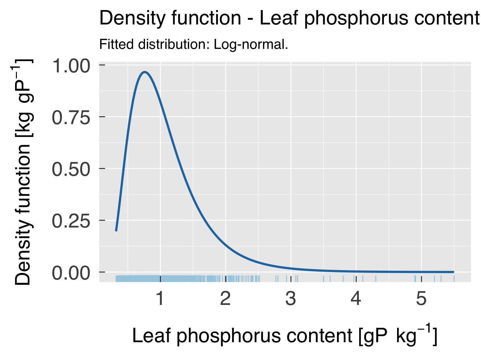
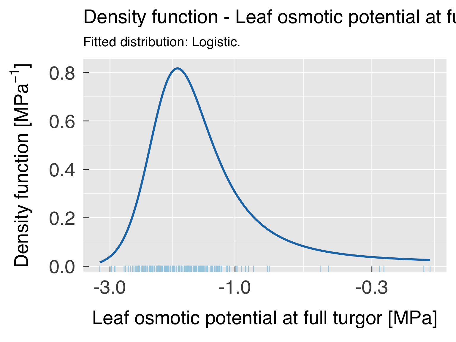
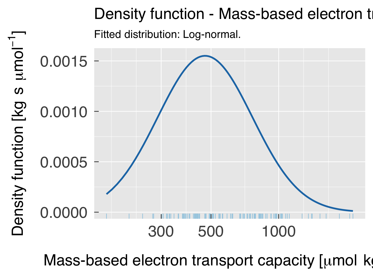
Plot trait density function by group
Here we plot the density functions of traits, separated by classes,
and along with the global distribution.
# Select reference data set for trade-off analysis
DataTRY    = switch( EXPR       = fit_taxon
                   , Individual = TidyTRY
                   , Species    = SpeciesTRY
                   , Genus      = GenusTRY
                   , stop("Invalid settings for variable \"fit_taxon\".")
                   )#end switch


# Find the number of sub-classes to test the model
CategDistr    = CategExtra %>%
   filter( ( (XYUse %in% "Colour") | (TraitID %in% 0L) | is.na(TraitID)) & (! duplicated(Class))) %>%
   mutate( Label = paste0(Class," (Not fitted)") )
CntCategDistr = nrow(CategDistr)


# Find out how many distribution plots we will make
xPlotDistr = which(try_trait$SMA & (try_trait$Name %in% InfoDistr$x))
CntDistr   = length(xPlotDistr)

# Initialise list with plots
gg_Distr = list()


CategSel    = is.finite(CategDistr$TraitID) & plot_categ_distrib
CategTrait  = sort(unique(CategDistr$TraitID[CategSel]))
for (ct in seq_along(CategTrait)){
   # Load settings for the classes.
   zTrait = CategTrait[ct]
   if (zTrait %in% 0L){
      zName  = "Cluster"
      zDesc  = "Data-based cluster class"
   }else{
      z      = match(zTrait,try_trait$TraitID)
      zName  = try_trait$Name   [z]
      zDesc  = try_trait$Desc   [z]
   }#end if (zTrait %in% 0L)
   zTitle = paste0("Trait distribution by ",tolower(zDesc))

   # Set path for this group of plots.
   categ_trdist_path = file.path(trdist_path,zName)

   # Select categories for this trait type.
   CategDistr = CategExtra %>%
      filter( (TraitID %in% zTrait) | is.na(TraitID)) %>%
      filter((! duplicated(Class))) %>%
      mutate(Label = ifelse(test=Class %in% "UKN",yes="UKN",no=NA_character_))
   CntCategDistr = nrow(CategDistr)


   # Select distribution statistics for this trait type
   InfoNow = InfoDistr %>%
      filter(TraitClass %in% c("All",zName)) %>%
      select(! TraitClass) %>%
      rename_at( vars(c("Class")), ~ c(zName)) %>%
      mutate(Label = NA_character_)

   # Loop through the SMA variables
   for (x in sequence(CntDistr)){
      # Load settings for the y axis.
      xIndex = xPlotDistr[x]
      xTrait = try_trait$TraitID[xIndex]
      xName  = try_trait$Name   [xIndex]
      xLower = paste0(xName,"_Lower")
      xUpper = paste0(xName,"_Upper")
      xDesc  = try_trait$Desc   [xIndex]
      xUnit  = try_trait$Unit   [xIndex]
      xTrans = try_trait$Trans  [xIndex]
      xTPlot = switch( EXPR = xTrans, log = "log10", neglog="neglog10",xTrans)

      # Select valid data for the x axis
      xSel = switch( EXPR     = xTrans
                   , identity = is.finite(DataTRY[[xName]])
                   , log      = DataTRY[[xName]] %gt% 0.
                   , neglog   = DataTRY[[xName]] %lt% 0.
                   , sqrt     = DataTRY[[xName]] %ge% 0.
                   , cbrt     = is.finite(DataTRY[[xName]])
                   , stop(paste0(" Invalid transformation for trait ",xName," (TraitID = ",xTrait,")."))
                   )#end switch

      # Subset data
      DataPlot = DataTRY %>%
         filter(xSel) %>%
         select_at(vars(c(xName,zName))) %>%
         mutate( across(c(zName), ~ifelse(.x %in% CategDistr$Class,.x,"UKN"))
               , across(c(zName), ~factor(.x,levels=CategDistr$Class))
               , density = NA_real_                                           )

      # Append dummy data with category ALL so legends can be merged.
      DataDummy = DataPlot[rep(1L,times=CntCategDistr),,drop=FALSE] %>%
         mutate( across(c(xName,"density"), ~ c(NA_real_))
               , across(c(zName), ~ factor(CategDistr$Class,levels=CategDistr$Class) ) )
      DataPlot    = rbind(DataPlot,DataDummy)
      CntDataPlot = nrow(DataPlot)

      # Plot only the variables with meaningful data
      PlotDistr   = CntDataPlot %gt% n_fit_min
      if (PlotDistr){
         cat0(" + Plot the trait distribution for ",xDesc," by ",zName,".")

         # Set path for this group of plots.
         dummy = dir.create(path=categ_trdist_path,recursive=TRUE,showWarnings=FALSE)

         # Find limits for plots.
         xLimit = range(DataPlot[[xName]],finite=TRUE)

         DistrPlot = tibble( x = rep(seq(from=xLimit[1L],to=xLimit[2L],length.out=n_predict),times=CntCategDistr)
                           , y = rep(NA_real_,times=CntCategDistr*n_predict)
                           , z = rep(CategDistr$Class,each=n_predict)
                           , d = rep(NA_character_,times=CntCategDistr*n_predict)
                           )#end tibble
         names(DistrPlot) = c(xName,"density",zName,"distr")

         # Turn classes into levels, so legends can be merged.
         DistrPlot = DistrPlot %>%
            mutate( across(c(zName), ~ factor(.x,levels = CategDistr$Class)) )

         # Generate consistent density functions
         zLoop = which(CategDistr$Class %in% unique(InfoNow[[zName]]))
         for (z in zLoop){
            # Identfy distribution
            zValue  = CategDistr$Class[z]
            zInfo   = which((InfoNow[[zName]] %in% zValue) & (InfoNow$x %in% xName))
            zDistr  = InfoNow$Distrib[zInfo]
            zFirst  = InfoNow$First  [zInfo]
            zSecond = InfoNow$Second [zInfo]
            zThird  = InfoNow$Third  [zInfo]
            if (zValue %in% "ALL"){
               zSel = DistrPlot[[zName]] %in% zValue
               rSel = DataPlot [[zName]] %in% "UKN"
            }else{
               zSel = DistrPlot[[zName]] %in% zValue
               rSel = DataPlot [[zName]] %in% zValue
            }#end if (zValue %in% "ALL")

            # Set the distribution
            DistrPlot$distr[zSel] = zDistr

            # Update label to include fitted distribution
            if (is.na(zDistr)){
               CategDistr$Label[z] = paste0(CategDistr$Class[z]," (Not fitted)")
            }else{
               CategDistr$Label[z] = paste0(CategDistr$Class[z]," (",str_to_sentence(zDistr),")")
            }#end if (is.na(zDistr))


            # Fit density according to the distribution.
            zFun = switch( zDistr
                         , "uniform"       = dunif
                         , "normal"        = dnorm
                         , "logistic"      = dlogis
                         , "skew-normal"   = sn::dsn
                         , "log-normal"    = dlnorm
                         , "neglog-normal" = dnlnorm
                         , "weibull"       = dweibull
                         , "gamma"         = dgamma
                         , NA_character_
                         )#end switch

            # Decide whether the distribution needs two or three parameters
            if (zDistr %in% "skew-normal"){
               if (any(zSel)) DistrPlot$density[zSel] = zFun(DistrPlot[[xName]][zSel],zFirst,zSecond,zThird)
               if (any(rSel)) DataPlot$density [rSel] = zFun(DataPlot [[xName]][rSel],zFirst,zSecond,zThird)
            }else if (! is.na(zDistr)){
               if (any(zSel)) DistrPlot$density[zSel] = zFun(DistrPlot[[xName]][zSel],zFirst,zSecond)
               if (any(rSel)) DataPlot$density [rSel] = zFun(DataPlot [[xName]][rSel],zFirst,zSecond)
            }#end if (zDistr %in% "skew-normal")
         }#end for (z in zLoop)

         # Prepare DataPlot to have random density locations below the curves
         DataPlot = DataPlot %>%
            mutate   ( density = density * runif(n=CntDataPlot) )

         # Find limits for density scale
         yLimit = range(DistrPlot$density,finite=TRUE)


         # Set categories for colours, lines and symbols
         colClasses        = CategDistr$Colour
         names(colClasses) = CategDistr$Class
         pchClasses        = CategDistr$Symbol
         names(pchClasses) = CategDistr$Class
         ltyClasses        = rep("solid",times=CntCategDistr)
         names(ltyClasses) = CategDistr$Class
         labClasses        = CategDistr$Label
         names(labClasses) = CategDistr$Class


         # Build the plot
         gg_now = ggplot()
         gg_now = gg_now + geom_point(data=DataPlot,aes_string(x=xName,y="density",colour=zName,shape=zName),size=1.5)
         gg_now = gg_now + geom_line(data=DistrPlot,aes_string(x=xName,y="density",colour=zName),size=1.25,inherit.aes = FALSE)
         gg_now = gg_now + scale_colour_manual  (values=colClasses,breaks=CategDistr$Class,labels=labClasses)
         gg_now = gg_now + scale_shape_manual   (values=pchClasses,breaks=CategDistr$Class,labels=labClasses)
         gg_now = gg_now + scale_linetype_manual(values=ltyClasses,breaks=CategDistr$Class,labels=labClasses)
         gg_now = gg_now + labs( x        = desc.unit(desc=xDesc,unit=untab[[xUnit]])
                               , y        = desc.unit(desc="Density function",unit=i.untab[[xUnit]])
                               , colour   = element_blank()
                               , fill     = element_blank()
                               , shape    = element_blank()
                               , title    = zTitle
                               , subtitle = LabelSubtitle
                               )#end labs
         gg_now = gg_now + theme_grey( base_size = gg_ptsz, base_family = "Helvetica",base_line_size = 0.5,base_rect_size =0.5)
         gg_now = gg_now + theme( axis.text.x       = element_text( size = gg_ptsz, margin = unit(rep(0.35,times=4),"cm"))
                                , axis.text.y       = element_text( size = gg_ptsz, margin = unit(rep(0.35,times=4),"cm"))
                                , plot.title        = element_text( size = gg_ptsz)
                                , plot.subtitle     = element_text( size = 0.7*gg_ptsz)
                                , axis.ticks.length = unit(-0.25,"cm")
                                , legend.position   = "bottom"
                                , legend.direction  = "horizontal"
                                )#end theme
         gg_now = gg_now + scale_x_continuous(trans=xTPlot,limits=xLimit)
         gg_now = gg_now + scale_y_continuous(trans="identity",limits=yLimit)
         gg_now = gg_now + guides(colour = guide_legend(nrow=2,byrow=TRUE))
         gg_now = gg_now + guides(shape  = guide_legend(nrow=2,byrow=TRUE))

         # Save plot in every format requested.
         for (d in sequence(ndevice)){
            f_output = paste0("DistrPlot_",xName,"_by-",zName,"_",base_suffix,".",gg_device[d])
            dummy = ggsave( filename = f_output
                          , plot     = gg_now
                          , device   = gg_device[d]
                          , path     = categ_trdist_path
                          , width    = gg_width
                          , height   = gg_height
                          , units    = gg_units
                          , dpi      = gg_depth
                          )#end ggsave
         }#end for (o in sequence(nout))

         # Write plot settings to the list.
         xzName = paste0(xName,"_",zName)
         gg_Distr[[xzName]] = gg_now
      }else{
         cat0(" + Skip plot for ",xDesc," by ",zDesc,": too few valid points.")

      }#end if (PlotSMA)
   }#end for (y in yloop)
}#end for (ct in seq_along(CategTrait)){


# If sought, plot images on screen
cnt_gg_Distr = length(gg_Distr)
if (gg_screen && (cnt_gg_Distr %gt% 0L)){
   gg_show = sort(sample.int(n=cnt_gg_Distr,size=min(cnt_gg_Distr,3L),replace=FALSE))
   gg_Distr[gg_show]
}#end if (gg_screen && (length(gg_Photo) %gt% 0L))
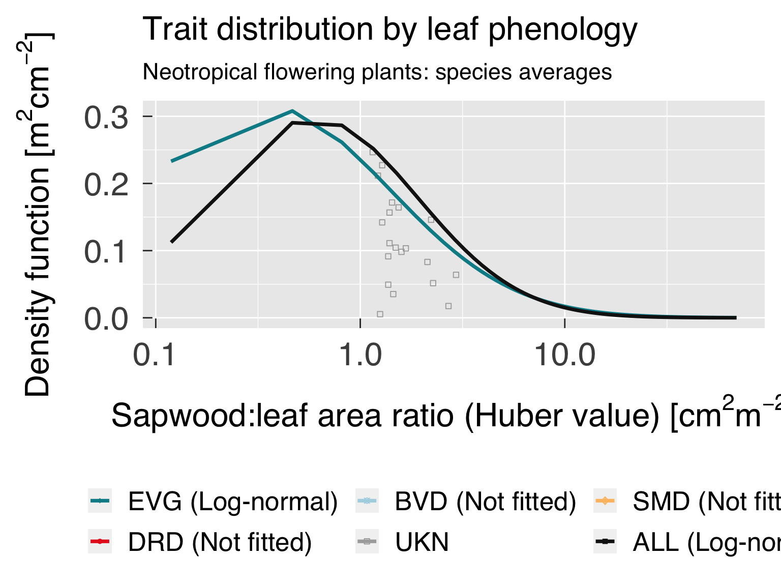
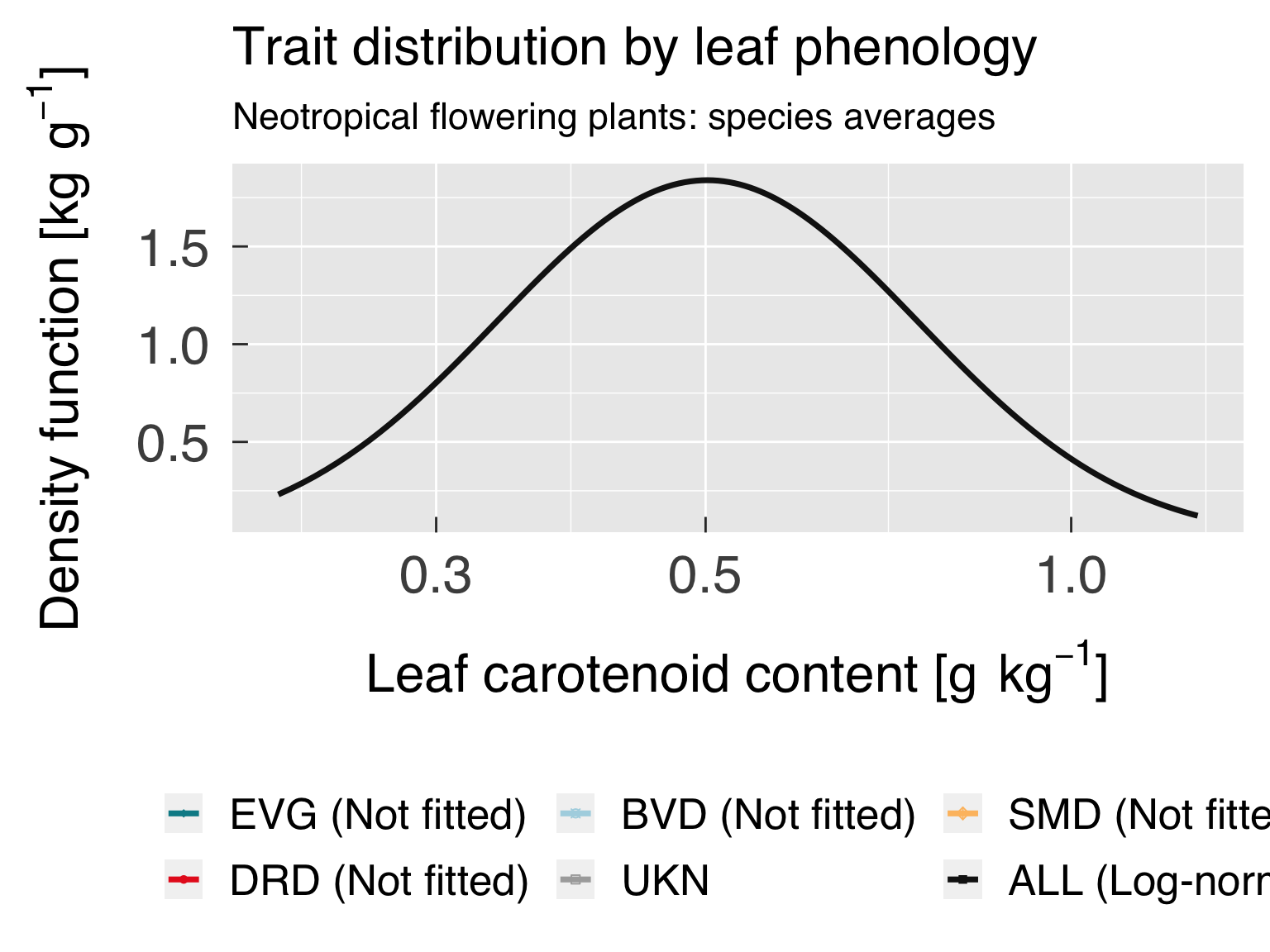
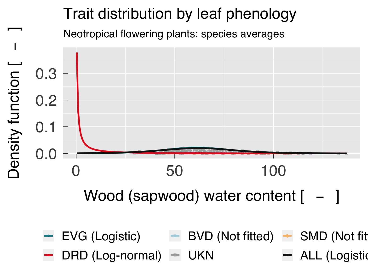
Plot trait density function by group using ridge (Joy Division)
plots
Here we plot the density functions of traits, separated by classes,
and along with the global distribution. We do not use the
ggridges package because we want the fitted distributions
to be plotted instead of the non-parametric distributions.
# Select reference data set for trade-off analysis
DataTRY    = switch( EXPR       = fit_taxon
                   , Individual = TidyTRY
                   , Species    = SpeciesTRY
                   , Genus      = GenusTRY
                   , stop("Invalid settings for variable \"fit_taxon\".")
                   )#end switch

# Find out how many distribution plots we will make
xPlotDistr = which(try_trait$SMA & (try_trait$Name %in% InfoDistr$x))
CntDistr   = length(xPlotDistr)

# Initialise list with plots
gg_Ridge = list()

CategInput  = CategExtra %>%
   filter( ( (XYUse %in% "Colour") | (TraitID %in% 0L) | is.na(TraitID) ) & (! duplicated(Class)) & plot_categ_ridge )
CategTrait  = sort(unique(CategInput$TraitID[CategSel]))
for (ct in seq_along(CategTrait)){
   # Load settings for the classes.
   zTrait = CategTrait[ct]
   if (zTrait %in% 0L){
      zName  = "Cluster"
      zDesc  = "Data-based cluster class"
   }else{
      z      = match(zTrait,try_trait$TraitID)
      zName  = try_trait$Name   [z]
      zDesc  = try_trait$Desc   [z]
   }#end if (zTrait %in% 0L)
   zTitle = paste0("Trait distribution by ",tolower(zDesc))

   # Set path for this group of plots.
   categ_trridge_path = file.path(trridge_path,zName)

   # Select categories for this trait type.
   CategDistr = CategInput %>%
      filter( (TraitID %in% zTrait) | (Class %in% "ALL") ) %>%
      filter((! duplicated(Class))) %>%
      mutate(Label = NA_character_)
   CntCategDistr = nrow(CategDistr)


   # Select distribution statistics for this trait type
   InfoNow = InfoDistr %>%
      filter(TraitClass %in% c("All",zName)) %>%
      select(! TraitClass) %>%
      rename_at( vars(c("Class")), ~ c(zName)) %>%
      mutate(Label = NA_character_)

   # Loop through the SMA variables
   for (x in sequence(CntDistr)){
      # Load settings for the y axis.
      xIndex = xPlotDistr[x]
      xTrait = try_trait$TraitID[xIndex]
      xName  = try_trait$Name   [xIndex]
      xLower = paste0(xName,"_Lower")
      xUpper = paste0(xName,"_Upper")
      xDesc  = try_trait$Desc   [xIndex]
      xUnit  = try_trait$Unit   [xIndex]
      xTrans = try_trait$Trans  [xIndex]
      xTPlot = switch( EXPR = xTrans, log = "log10", neglog="neglog10",xTrans)

      # Select valid data for the x axis
      xSel = switch( EXPR     = xTrans
                   , identity = is.finite(DataTRY[[xName]])
                   , log      = DataTRY[[xName]] %gt% 0.
                   , neglog   = DataTRY[[xName]] %lt% 0.
                   , sqrt     = DataTRY[[xName]] %ge% 0.
                   , cbrt     = is.finite(DataTRY[[xName]])
                   , stop(paste0(" Invalid transformation for trait ",xName," (TraitID = ",xTrait,")."))
                   )#end switch

      # Subset data
      DataPlot = DataTRY %>%
         filter(xSel) %>%
         select_at(vars(c(xName,zName))) %>%
         mutate( across(c(zName), ~ifelse(.x %in% CategDistr$Class,.x,"ALL"))
               , across(c(zName), ~factor(.x,levels=CategDistr$Class))
               , offset  = NA_real_
               , density = NA_real_                                           )

      # Append dummy data with category ALL so legends can be merged.
      DataDummy = DataPlot[rep(1L,times=CntCategDistr),,drop=FALSE] %>%
         mutate( across(c(xName,"offset","density"), ~ c(NA_real_))
               , across(c(zName), ~ factor(CategDistr$Class,levels=CategDistr$Class) ) )
      DataPlot    = rbind(DataPlot,DataDummy)
      CntDataPlot = nrow(DataPlot)

      # Plot only the variables with meaningful data
      PlotDistr   = CntDataPlot %gt% n_fit_min
      if (PlotDistr){
         cat0(" + Plot the trait distribution for ",xDesc," by ",zName,".")

         # Set path for this group of plots.
         dummy = dir.create(path=categ_trridge_path,recursive=TRUE,showWarnings=FALSE)

         # Find limits for plots.
         xLimit = range(DataPlot[[xName]],finite=TRUE)

         DistrPlot = tibble( x  = rep(seq(from=xLimit[1L],to=xLimit[2L],length.out=n_predict),times=CntCategDistr)
                           , l  = rep(NA_real_,times=CntCategDistr*n_predict)
                           , u  = rep(NA_real_,times=CntCategDistr*n_predict)
                           , z  = rep(CategDistr$Class,each=n_predict)
                           , d  = rep(NA_character_,times=CntCategDistr*n_predict)
                           )#end tibble
         names(DistrPlot) = c(xName,"offset","density",zName,"distr")

         # Turn classes into levels, so legends can be merged.
         DistrPlot = DistrPlot %>%
            mutate( across(c(zName), ~ factor(.x,levels = CategDistr$Class)) )

         # Generate consistent density functions
         zLoop = which(CategDistr$Class %in% unique(InfoNow[[zName]]))
         onow  = -1L
         for (z in zLoop){
            # Update offset
            onow = onow + 1L

            # Identfy distribution
            zValue  = CategDistr$Class[z]
            zInfo   = which((InfoNow[[zName]] %in% zValue) & (InfoNow$x %in% xName))
            zDistr  = InfoNow$Distrib[zInfo]
            zFirst  = InfoNow$First  [zInfo]
            zSecond = InfoNow$Second [zInfo]
            zThird  = InfoNow$Third  [zInfo]
            if (zValue %in% "ALL"){
               zSel = DistrPlot[[zName]] %in% zValue
               rSel = DataPlot [[zName]] %in% "UKN"
            }else{
               zSel = DistrPlot[[zName]] %in% zValue
               rSel = DataPlot [[zName]] %in% zValue
            }#end if (zValue %in% "ALL")

            # Set the distribution
            DistrPlot$distr[zSel] = zDistr

            # Update label to include fitted distribution
            if (is.na(zDistr)){
               CategDistr$Label[z] = paste0(CategDistr$Class[z]," (Not fitted)")
            }else{
               CategDistr$Label[z] = paste0(CategDistr$Class[z]," (",str_to_sentence(zDistr),")")
            }#end if (is.na(zDistr))


            # Fit density according to the distribution.
            zFun = switch( zDistr
                         , "uniform"       = dunif
                         , "normal"        = dnorm
                         , "logistic"      = dlogis
                         , "skew-normal"   = sn::dsn
                         , "log-normal"    = dlnorm
                         , "neglog-normal" = dnlnorm
                         , "weibull"       = dweibull
                         , "gamma"         = dgamma
                         , NA_character_
                         )#end switch

            # Append offsets
            if (any(zSel)) DistrPlot$offset[zSel] = onow
            if (any(rSel)) DataPlot$offset [rSel] = onow

            # Decide whether the distribution needs two or three parameters
            if (zDistr %in% "skew-normal"){
               if (any(zSel)) DistrPlot$density[zSel] = zFun(DistrPlot[[xName]][zSel],zFirst,zSecond,zThird)
               if (any(rSel)) DataPlot$density [rSel] = zFun(DataPlot [[xName]][rSel],zFirst,zSecond,zThird)
            }else if (! is.na(zDistr)){
               if (any(zSel)) DistrPlot$density [zSel] = zFun(DistrPlot[[xName]][zSel],zFirst,zSecond)
               if (any(rSel)) DataPlot$density  [rSel] = zFun(DataPlot [[xName]][rSel],zFirst,zSecond)
            }#end if (zDistr %in% "skew-normal")
         }#end for (z in zLoop)

         # Find scaling factor for all densities, allowing a bit of overlap between the curves
         DensityMax = 0.6 * max(DistrPlot$density,na.rm=TRUE)
         DistrPlot  = DistrPlot %>%
            mutate( ridge = offset + density / DensityMax)
         DataPlot   = DataPlot %>%
            mutate( ridge = offset + density / DensityMax * runif(n=CntDataPlot))

         # Find limits for density scale
         yLimit  = range(c(DistrPlot$offset,DistrPlot$ridge),finite=TRUE)
         yAt     = seq_along(zLoop) - 1L
         yLabels = CategDistr$Label[zLoop]


         # Set categories for colours, lines and symbols
         colClasses        = CategDistr$Colour
         names(colClasses) = CategDistr$Class
         bgClasses         = alpha(colClasses,alpha=0.4)
         names(bgClasses)  = CategDistr$Class
         pchClasses        = CategDistr$Symbol
         names(pchClasses) = CategDistr$Class
         ltyClasses        = rep("solid",times=CntCategDistr)
         names(ltyClasses) = CategDistr$Class
         labClasses        = CategDistr$Label
         names(labClasses) = CategDistr$Class


         # Build the plot
         gg_now = ggplot()
         gg_now = gg_now + geom_ribbon( data        = DistrPlot
                                      , mapping     = aes_string(x=xName,ymin="offset",ymax="ridge",colour=zName,fill=zName)
                                      , size        = 1.25
                                      , inherit.aes = FALSE
                                      , show.legend = FALSE
                                      )#end geom_ribbon
         gg_now = gg_now + geom_point( data        = DataPlot
                                     , mapping     = aes_string(x=xName,y="ridge",colour=zName,shape=zName)
                                     , size        = 1.5
                                     , show.legend = FALSE
                                     )#end geom_point
         gg_now = gg_now + scale_colour_manual  (values=colClasses,breaks=CategDistr$Class,labels=labClasses)
         gg_now = gg_now + scale_fill_manual    (values=bgClasses ,breaks=CategDistr$Class,labels=labClasses)
         gg_now = gg_now + scale_shape_manual   (values=pchClasses,breaks=CategDistr$Class,labels=labClasses)
         gg_now = gg_now + scale_linetype_manual(values=ltyClasses,breaks=CategDistr$Class,labels=labClasses)
         gg_now = gg_now + labs( x        = desc.unit(desc=xDesc,unit=untab[[xUnit]])
                               , y        = element_blank()
                               , colour   = element_blank()
                               , fill     = element_blank()
                               , shape    = element_blank()
                               , title    = zTitle
                               , subtitle = LabelSubtitle
                               )#end labs
         gg_now = gg_now + theme_grey( base_size = gg_ptsz, base_family = "Helvetica",base_line_size = 0.5,base_rect_size =0.5)
         gg_now = gg_now + theme( axis.text.x       = element_text( size = gg_ptsz, margin = unit(rep(0.35,times=4),"cm"))
                                , axis.text.y       = element_text( size = gg_ptsz, margin = unit(rep(0.35,times=4),"cm"))
                                , plot.title        = element_text( size = gg_ptsz)
                                , plot.subtitle     = element_text( size = 0.7*gg_ptsz)
                                , axis.ticks.length = unit(-0.25,"cm")
                                , legend.position   = "bottom"
                                , legend.direction  = "horizontal"
                                )#end theme
         gg_now = gg_now + scale_x_continuous(trans=xTPlot,limits=xLimit)
         gg_now = gg_now + scale_y_continuous(trans="identity",limits=yLimit,breaks=yAt,labels=yLabels)
         gg_now = gg_now + guides(colour = guide_legend(nrow=2,byrow=TRUE))
         gg_now = gg_now + guides(shape  = guide_legend(nrow=2,byrow=TRUE))

         # Save plot in every format requested.
         for (d in sequence(ndevice)){
            f_output = paste0("RidgePlot_",xName,"_by-",zName,"_",base_suffix,".",gg_device[d])
            dummy = ggsave( filename = f_output
                          , plot     = gg_now
                          , device   = gg_device[d]
                          , path     = categ_trridge_path
                          , width    = gg_width
                          , height   = gg_height
                          , units    = gg_units
                          , dpi      = gg_depth
                          )#end ggsave
         }#end for (o in sequence(nout))

         # Write plot settings to the list.
         xzName = paste0(xName,"_",zName)
         gg_Ridge[[xzName]] = gg_now
      }else{
         cat0(" + Skip plot for ",xDesc," by ",zDesc,": too few valid points.")

      }#end if (PlotSMA)
   }#end for (y in yloop)
}#end for (ct in seq_along(CategTrait)){


# If sought, plot images on screen
cnt_gg_Ridge = length(gg_Ridge)
if (gg_screen && (cnt_gg_Ridge %gt% 0L)){
   gg_show = sort(sample.int(n=cnt_gg_Ridge,size=min(cnt_gg_Ridge,3L),replace=FALSE))
   gg_Ridge[gg_show]
}#end if (gg_screen && (length(gg_Ridge) %gt% 0L))